Data Wrangling Exercise 2

Group, Summarize, and Join Data Frames

In this exercise, we’ll continue to work with the pop-quiz data using the following techniques:

group & summarize
table joins

Setup

Load the packages we’ll be using:

library(readr)
library(dplyr)
library(ggplot2)
library(stringr)
library(conflicted)
conflicts_prefer(
  dplyr::select,
  dplyr::filter,
  dplyr::arrange
)

We’ll continue to work with the pop-quiz data we saw in the first exercise. (Note how we can cleanup the column names in the same expression that imports the file):

ss_fn <- here::here("./exercises/data/student_scores.tsv")
ss_nn_tbl <- readr::read_tsv(file = ss_fn, show_col_types = FALSE) |> 
  rename_with(tolower, everything()) |>
  rename_with(~ str_replace_all(., " ", "_"), everything())
head(ss_nn_tbl)

For this exercise, we’ll also continue to work with the first quiz only:

ss_q1_tbl <- ss_nn_tbl |> 
  select(name, section, treatment, quiz_01)
head(ss_q1_tbl)

Group and Summarize

Let’s compute the number of students per section. We start by grouping the rows by section:

ss_q1_tbl |> 
  group_by(section)

Note: Simply grouping rows with group_by() doesn’t do anything useful!

You have to follow it up with something else (usually summarize()).

To return the number of rows per group, we can define a new column using n().

ss_q1_tbl |> 
  group_by(section) |> 
  summarize(num_students = n())

Functions you can use in summarize()

What gets fed into summarize() are groups of rows (one at a time).

Hence, when you define columns in summarize(), you have to use functions that can receive multiple values and return just one (i.e., aggregate functions). Common examples include n(), mean(), sum(), max(), first(), etc. See the ‘Summary Functions’ on the dplyr cheatsheet for others.

Next, compute the average score on Quiz 1 by section:

ss_q1_tbl |> 
  group_by(section) |> 
  summarize(quiz_01_avg = mean(quiz_01, na.rm = TRUE))

CHALLENGE

Compute the average score on Quiz 1 by treatment group. (solution)

ss_q1_tbl |> 
  group_by(treatment) |> 
  summarize(quiz_01_avg = mean(quiz_01, na.rm = TRUE))

Group on Multiple Columns

We can group by more than one column. For example, to view the number of students in each treatment group per section:

ss_q1_tbl |> 
  group_by(section, treatment) |> 
  summarize(num_students = n())

`summarise()` has grouped output by 'section'. You can override using the
`.groups` argument.

CHALLENGE

Compute the number of students per treatment group and sex. (solution)

ss_nn_tbl |> 
  group_by(treatment, sex) |> 
  summarize(num_students = n())

`summarise()` has grouped output by 'treatment'. You can override using the
`.groups` argument.

Join Tables

Joining tables together is extremely useful for wrangling data!

Let’s bring in a table with more info about the discussion sections:

sect_info_fn <- here::here("exercises/data/section_info.tsv")
sect_info_tbl <- read_tsv(sect_info_fn)

Rows: 4 Columns: 4
── Column specification ────────────────────────────────────────────────────────
Delimiter: "\t"
chr  (3): section, ta, day
time (1): time

ℹ Use `spec()` to retrieve the full column specification for this data.
ℹ Specify the column types or set `show_col_types = FALSE` to quiet this message.

sect_info_tbl

To join tables on a common column, you can use dplyr::left_join():

ss_q1_sect_tbl <- ss_q1_tbl |> 
  left_join(sect_info_tbl, by = "section")
ss_q1_sect_tbl

Use the New Columns for Summaries

Once the tables are joined, the new columns are available for use.

For each Teaching Assistant, compute the number of students, and their avg on quiz 1.

ss_q1_sect_tbl |> 
  group_by(ta) |> 
  summarise(count = n(), 
            avg_score = mean(quiz_01, na.rm = TRUE))

CHALLENGE

How many students have discussion on each day of the week? (solution)

ss_q1_sect_tbl |> 
  group_by(day) |> 
  summarise(count = n())

Based on Quiz 1, is there any evidence to support the theory that students who have discussion section earlier in the day tend to have better learning outcomes? (solution)

## Is there any evidence to support the theory that students who have discussion section
## earlier in the day tend to have better learning outcomes?

ss_q1_sect_tbl |> 
  group_by(time) |> 
  summarise(avg_score = mean(quiz_01, na.rm = TRUE))

ggplot(ss_q1_sect_tbl, aes(y = quiz_01, x = time)) +
  geom_point() +
  labs(title = "Quiz 1 Scores by Discussion Section Hour")

Warning: Removed 20 rows containing missing values or values outside the scale range
(`geom_point()`).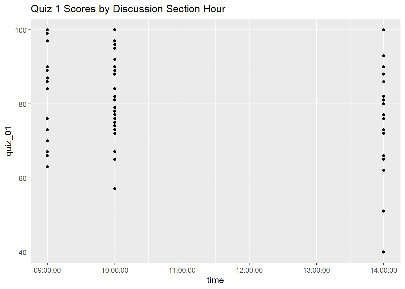

ggplot(ss_q1_sect_tbl, aes(y = quiz_01, x = as.character(time))) +
  geom_boxplot() +
  labs(title = "Quiz 1 Scores by Discussion Section Hour")

Warning: Removed 20 rows containing non-finite outside the scale range
(`stat_boxplot()`).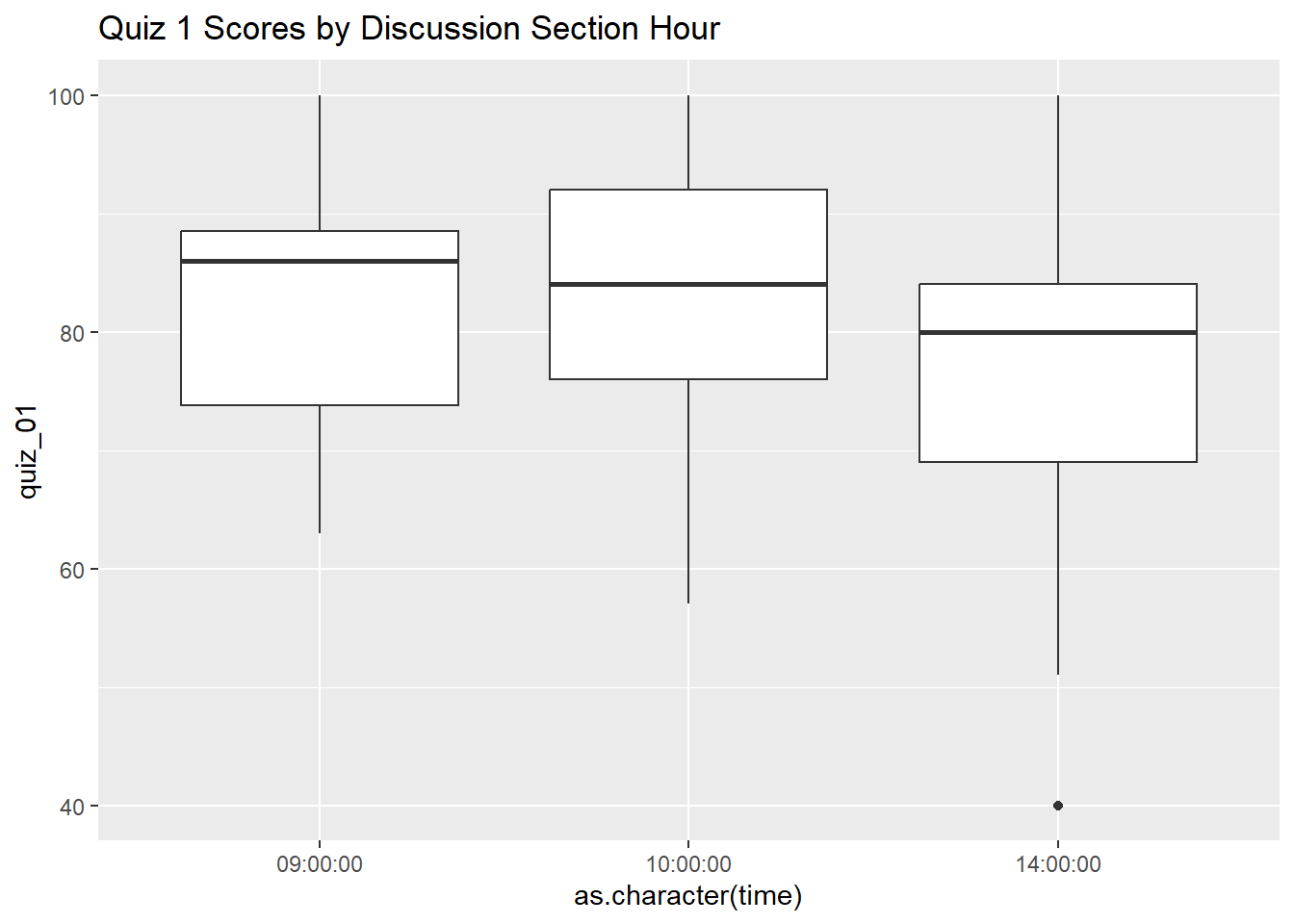

## Note: While the averages for the 9:00a and 10:00a discussion sections look
## quite a bit higher than the 2:00p section, when we look at the spread it
## appears the 2:00p average might have been brought down by two outliers.

DONE!

Remember to render your Quarto document so you have a pretty HTML file to keep for future reference.