Some of My R Work

degday

Compute degree days in R
https://ucanr-igis.github.io/degday/

uasimg

Data management utilities for drone mapping
https://ucanr-igis.github.io/uasimg/

caladaptR

Bring climate data from Cal-Adapt into R using the API
https://ucanr-igis.github.io/caladaptr/

T-Locoh

Homerange and spatial-temporal pattern analysis for wildlife tracking data
http://tlocoh.r-forge.r-project.org/

Shiny Apps

Chill Portions Under Climate Change Calculator
https://ucanr-igis.shinyapps.io/chill/

Drone Mission Planner for Reforestation Monitoring Protocol
https://ucanr-igis.shinyapps.io/uav_stocking_survey/

Stock Pond Volume Calculator
https://ucanr-igis.shinyapps.io/PondCalc/

Pistachio Nut Growth Calculator
https://ucanr-igis.shinyapps.io/pist_gdd/

Workshop Goals

Gain a better understanding of the fundamentals of data wrangling
Be able to find the packages and functions that can do what you need
Grow your library of working code recipes
Be better equipped to trouble-shoot your code
Come out slightly higher on the learning curve!

Data Wrangling: What do we mean?

Whatever is needed to get your data frame ready
for the function(s) you want to use for analysis and visualization.

Also called: data munging, data manipulation, data transformation, etc.

Operations

Data wrangling often includes some combination of:

dropping columns
renaming columns
changing the order of columns
creating new columns with an expression
filtering rows
sorting rows
going from 'long' to 'wide' formats
joining data frames based on a common field
merging / stacking data frames together
splitting tables
aggregating rows into groups
splitting columns into new columns / rows

Outline

Developing a strategy

What is tidy data?
Working backwards

R Methods

Importing data
Subsetting rows and columns
Creating new columns
Class conversions: text, dates, numbers, units
Splitting columns
Joining tables
Grouping and summarizing rows
Dealing with missing values
Reshaping data

More advanced tasks

Wrangling really large data
Flattening nested data
Splitting flat data into relational tables
Reading and writing databases
??

Planning Your Data Wrangling Strategy

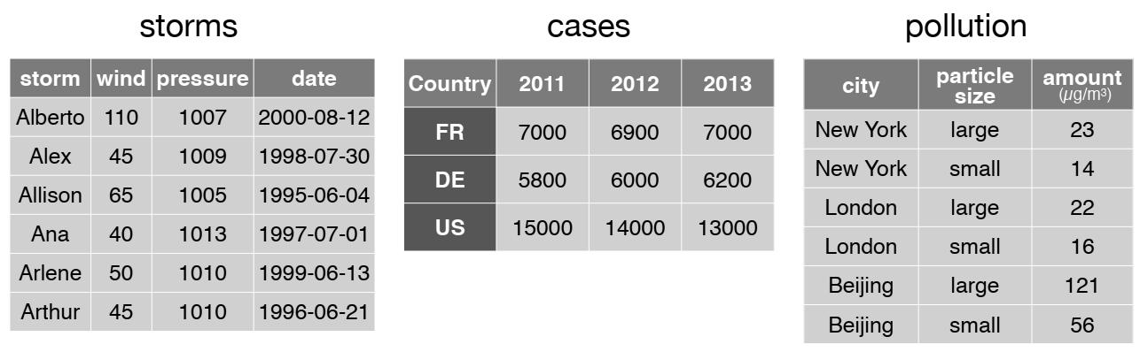
What is "tidy data"?

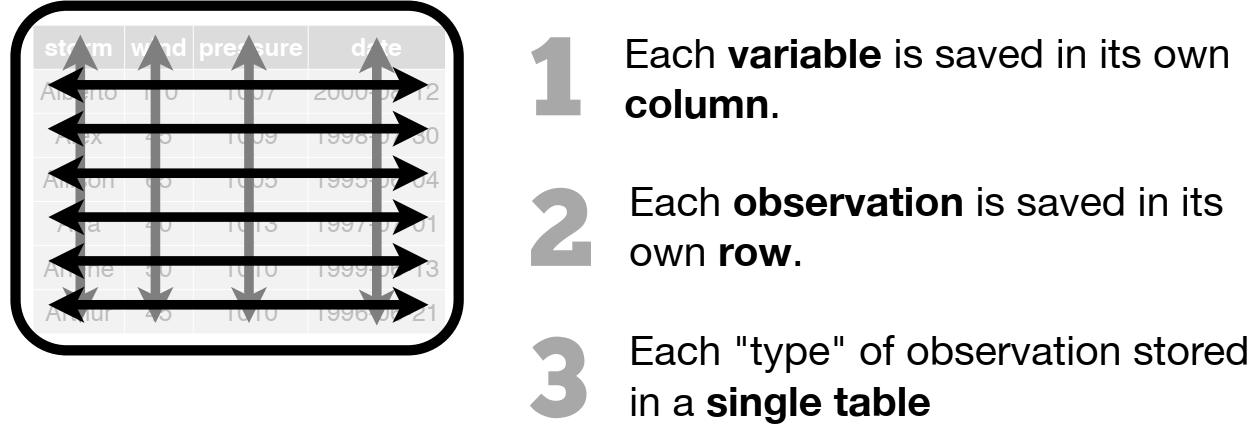
Wickham, H. (2014). Tidy data. Journal of statistical software, 59, 1-23. https://doi.org/10.18637/jss.v059.i10

Are these data 'tidy'?

Do I have to use tidy data?

Advantages of tidy data

computers programs like it!
makes data wrangling code really efficient
many, many R developers are developing 'tidy-ready' functions in their packages

Reasons not to use tidy data

if your data are not rectangular
designing a table for human consumption
simple rowwise calculation (e.g. t1 - t2)
if the stats / analysis function requires something specific

Data Wrangling Methods

Tidyverse

Install them all at once:

install.packages("tidyverse")

For the complete list of all the tidyverse packages, see:

https://tidyverse.tidyverse.org/

Core Packages

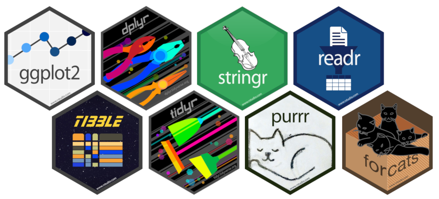
Load core packages all at once:

library(tidyverse)

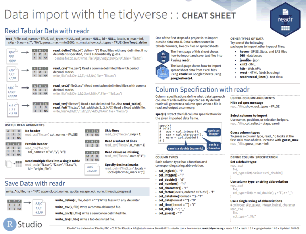
Better Ways to Import Tabular Data

These packages allow you to:

import tabular data in different formats
skip rows that don't actually contain data
specify whether the file contains a header
rename columns as part of the importing
specify the data type for each column

Example:

library(readxl)
my_tbl = read_xlsx(path = "plot_data.xlsx", 
                   sheet = "Sheet2",
                   skip = 3,
                   col_names = c("plot_num", "date", "species", "count"),
                   col_types = c("text", "date", "text", "integer"))

Explore Data

So whatdya we got here?

Structure

dim()
nrow()
ncol()

str()

Preview the data

head()
View()

dplyr::glimpse()

Distribution and Frequency

summary()

## Discrete values
unique()
table()

Plots

hist()

plot(x,y)
qqplot()

Missing Values

is.na()
anyNA()

Little bit of everything

summary()

Data Wrangling with `dplyr`

Cheatsheet

An alternative (usually better) way to wrangle data frames than base R.

Best way to familiarize yourself - explore the cheat sheet:

Popular `dplyr` Functions

Row and Column Manipulations

subset rows	filter(), slice()
order rows	arrange()
pick column(s)	select(), pull()
add new columns	mutate()

Subset Rows

The two functions most commonly used to subset rows include filter() and slice().

use filter() to subset based on a logical expressions
use slice() to subset based on indices

Logical expressions you can use in filter() include:

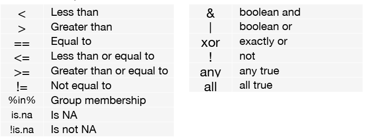
Chaining dplyr functions

Most dplyr functions take a tibble as the first argument , and return a tibble.

This makes them very pipe friendly.

Example

Look at the storms tibble:

library(dplyr)
head(storms)

## # A tibble: 6 × 13
##   name   year month   day  hour   lat  long status       category  wind pressure
##   <chr> <dbl> <dbl> <int> <dbl> <dbl> <dbl> <fct>           <dbl> <int>    <int>
## 1 Amy    1975     6    27     0  27.5 -79   tropical de…       NA    25     1013
## 2 Amy    1975     6    27     6  28.5 -79   tropical de…       NA    25     1013
## 3 Amy    1975     6    27    12  29.5 -79   tropical de…       NA    25     1013
## 4 Amy    1975     6    27    18  30.5 -79   tropical de…       NA    25     1013
## 5 Amy    1975     6    28     0  31.5 -78.8 tropical de…       NA    25     1012
## 6 Amy    1975     6    28     6  32.4 -78.7 tropical de…       NA    25     1012
## # ℹ 2 more variables: tropicalstorm_force_diameter <int>,
## #   hurricane_force_diameter <int>

Filter out only the records for category 3 or higher storms

storms |> 
  select(name, year, month, category) |>     ## select the columns we need
  filter(category >= 3)                      ## select just the rows we want

## # A tibble: 1,262 × 4
##    name      year month category
##    <chr>    <dbl> <dbl>    <dbl>
##  1 Caroline  1975     8        3
##  2 Caroline  1975     8        3
##  3 Eloise    1975     9        3
##  4 Eloise    1975     9        3
##  5 Gladys    1975    10        3
##  6 Gladys    1975    10        3
##  7 Gladys    1975    10        4
##  8 Gladys    1975    10        4
##  9 Gladys    1975    10        3
## 10 Belle     1976     8        3
## # ℹ 1,252 more rows

dplyr functions generally allow you to enter column names without quotes.

`stringr`

Cheatsheet

Replace characters:

str_replace_all(string = "The Quick Brown Fox",
                pattern = " ",
                replacement = "_")

## [1] "The_Quick_Brown_Fox"

Split a character into two:

str_split_1("horse, cart, buggy", pattern = ",")

## [1] "horse"  " cart"  " buggy"

Trim white space:

str_trim("  123 California Hall   ", side = "both")

## [1] "123 California Hall"

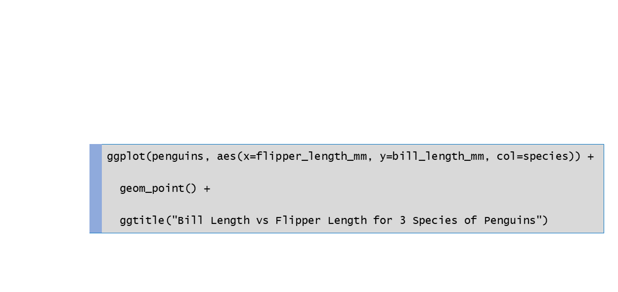
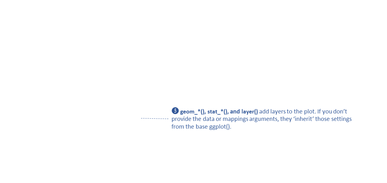
ggplot

ggplot2 is an extremely popular plotting package for R.

ggplots are constructed using the ‘grammar of graphics’ paradigm.

library(ggplot2)
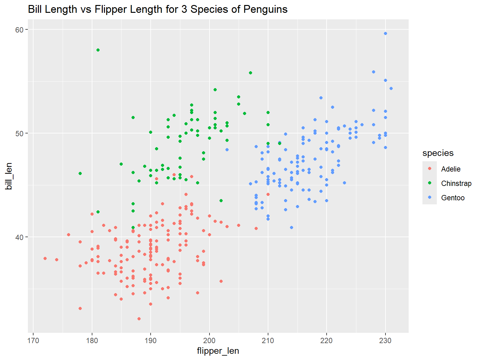
ggplot(penguins, aes(x = flipper_len, y = bill_len, color = species)) +
  geom_point() +
  ggtitle("Bill Length vs Flipper Length for 3 Species of Penguins")

Maping Columns to Symbology Properties with `aes()`

ggplot(penguins, aes(x = flipper_length_mm , y = bill_length_mm , color = species)) +
  geom_point() +
  ggtitle("Bill Length vs Flipper Length for 3 Species of Penguins")

aes() sets the default source for each visual property (or aesthetic) of the plot layers
- note you don't need to put column names in quotes
some common visual properties:

x - where it falls along the x-axis
y - where it falls along the y-axis
color
fill
size
linewidth

which visual properties are needed depends on the geom_xxxx() functions you use
only put in aes() the visual properties you want linked to the data

Geoms

geom_xxxx() functions draw layers on the plot canvas
drawn from the bottom up
some common geoms:

geom_point()

geom_bar()

geom_boxplot()

geom_histogram()

visual properties can be linked to a column in the data frame or manually specified

geom_point(col = pop_size)

geom_point(col = "red")

visual properties are inherited (from aes())
each geom has default color palettes and legend settings

Example:

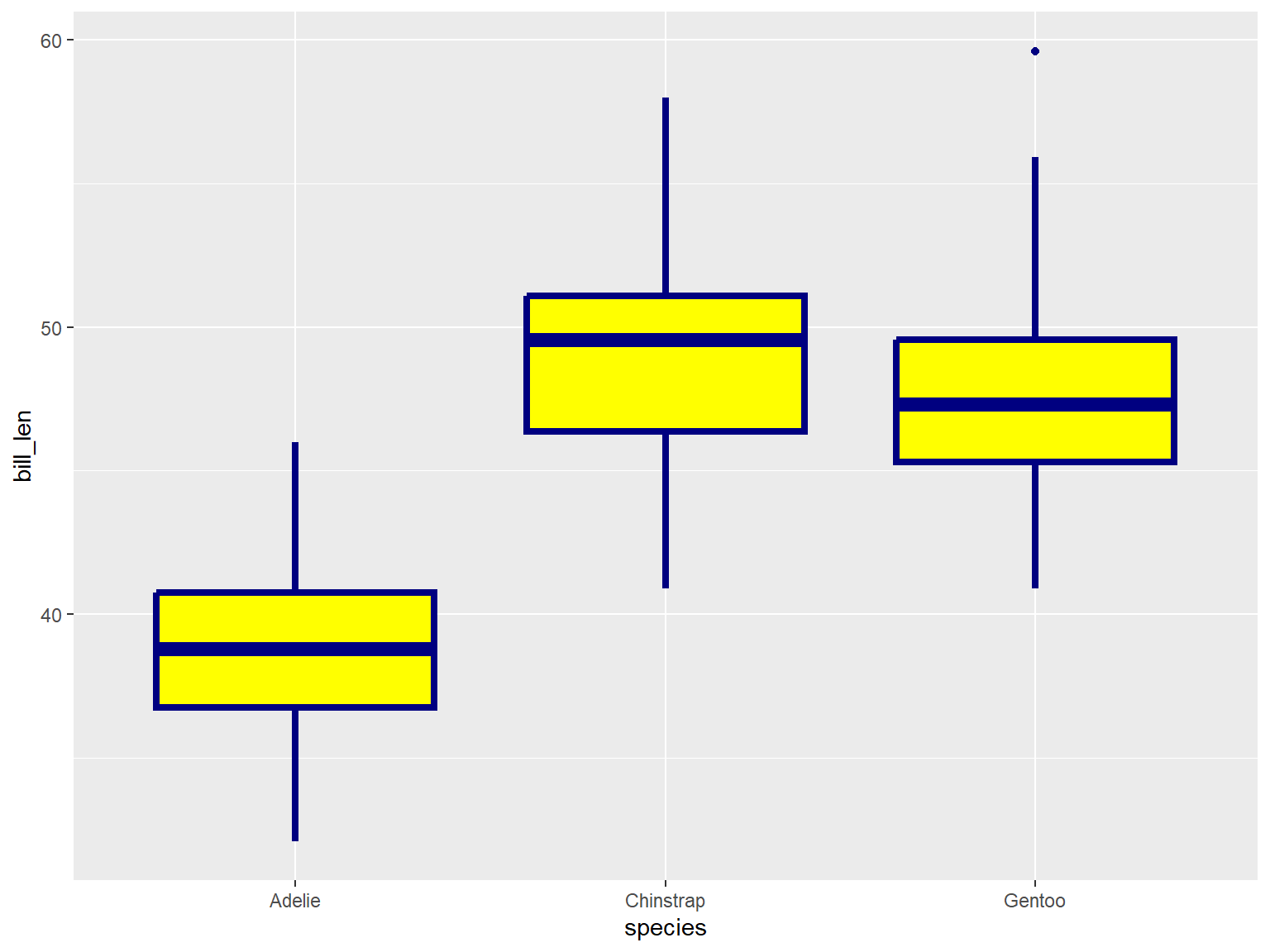
In the example below, note where geom_boxplot() gets its visual properties:

x and y are linked to columns in the dataframe and inherited from aes()
color, fill, and size are manually specified

ggplot(penguins, aes(x = species, y = bill_len)) +
  geom_boxplot(color = "navy", fill = "yellow", size = 1.5)

## Warning: Removed 2 rows containing non-finite outside the scale range
## (`stat_boxplot()`).

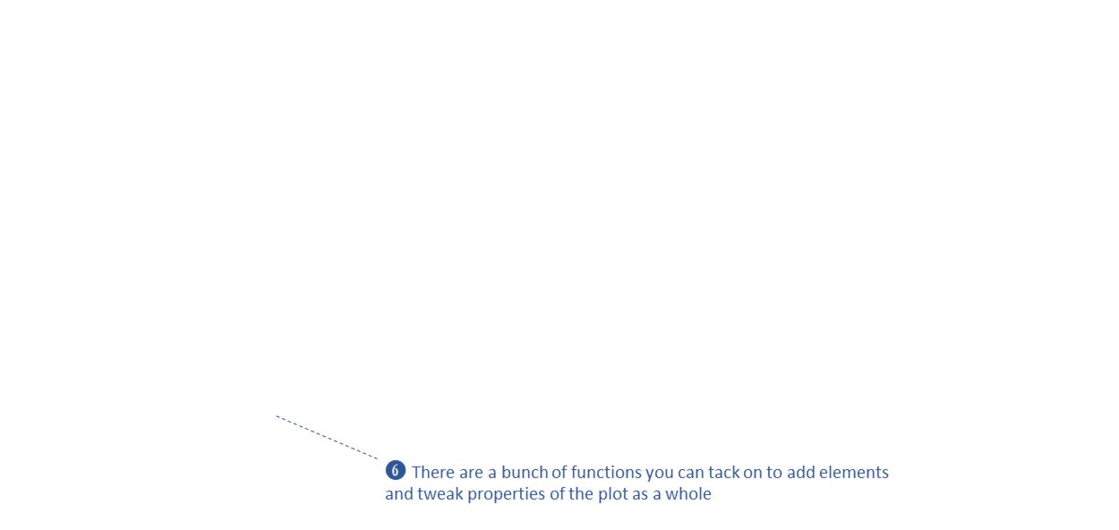
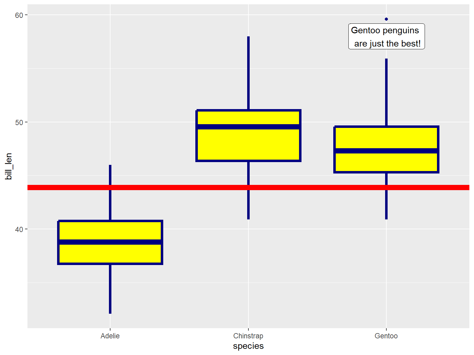
Adding visual elements to a plot

geom_xxxx() functions can also be used to add other graphic elements:

ggplot(penguins, aes(x = species, y = bill_len)) +
  geom_boxplot(color = "navy", fill = "yellow", size = 1.5) +
  geom_hline(yintercept = 43.9, linewidth = 3, color="red") +
  geom_label(x = 3, y = 58, label = "Gentoo penguins \n are just the best!")

## Warning: Removed 2 rows containing non-finite outside the scale range
## (`stat_boxplot()`).

Exercise 1

In this exercise, we will:

import some messy survey data from Excel
import, clean, and visualize weekly pop-quiz scores

improve column names
subset columns
plot distributions
sort and subset rows
compute new columns
resample columns
split columns

This exercise will be done in an Quarto Notebook!

https://posit.cloud/content/11134060

Highlights of Exercise 1

Data wrangling starts when you import data

use readxl or readr

Exploring what you got

ggplot() can split up the data for visualization
base R functions: dim(), summarize(), table()
head(), View()

Renaming columns

one-by-one: use rename() or select()
apply a function to several columns at once: use rename_with()

Subsetting rows and columns

select()
filter(), slice()

Exploring the top and bottom values

arrange()
slice_max(), slice_min()

Add or modify columns: mutate() with:

any vectorized function or operator
min_rank()
if_else()
case_when()

Splitting columns

mutate + stringr::str_split_i()
tidyr::separate_wider_delim() - more flexible

tidy-select Expressions

tidy-select functions can be used to specify columns in a data frame.

These expressions can be used wherever you need to specify columns, including:

select()
rename_with()
mutate(across())

Examples

-student_id	all columns except age
quiz_01:quiz10	all columns between `quiz_01` and `quiz_10`
starts_with("Quiz")	all columns that start with 'Quiz'
contains('cm')	column names that contain 'cm'
all_of(c('major', 'gpa')) any_of(c('major', 'gpa'))	column names stored in a vector
last_col()	last column
everything()	all columns

More info:
https://tidyselect.r-lib.org/

Data File Formats

There are better options for storing data than csv.

RDS - R's native format
TSV - tab-separated values
Feather - column based, binary, cross-platform
Parquet - column based, binary, cross-platform
DuckDB, sqlite, PostgresSQL, MySQL - relational databases

Group and Summarize

Step 1 (optional): group rows (i.e., change the unit of analysis)	`group_by()`
Step 2: Compute summaries for each group of rows	Add summary columns with `summarize()` Aggregate functions available: `n(), mean(), median(), sum(), sd(), IQR(), first(),` etc.

Example:

library(dplyr)
head(storms)

## # A tibble: 6 × 13
##   name   year month   day  hour   lat  long status       category  wind pressure
##   <chr> <dbl> <dbl> <int> <dbl> <dbl> <dbl> <fct>           <dbl> <int>    <int>
## 1 Amy    1975     6    27     0  27.5 -79   tropical de…       NA    25     1013
## 2 Amy    1975     6    27     6  28.5 -79   tropical de…       NA    25     1013
## 3 Amy    1975     6    27    12  29.5 -79   tropical de…       NA    25     1013
## 4 Amy    1975     6    27    18  30.5 -79   tropical de…       NA    25     1013
## 5 Amy    1975     6    28     0  31.5 -78.8 tropical de…       NA    25     1012
## 6 Amy    1975     6    28     6  32.4 -78.7 tropical de…       NA    25     1012
## # ℹ 2 more variables: tropicalstorm_force_diameter <int>,
## #   hurricane_force_diameter <int>

For each month, how many storm observations are saved in the data frame

storms |> 
  select(name, year, month, category) |>    ## select the columns we need
  group_by(month) |>                        ## group the rows by month
  summarize(num_storms = n())               ## for each group, report the count

## # A tibble: 10 × 2
##    month num_storms
##    <dbl>      <int>
##  1     1         70
##  2     4         66
##  3     5        201
##  4     6        809
##  5     7       1651
##  6     8       4442
##  7     9       7778
##  8    10       3138
##  9    11       1170
## 10    12        212

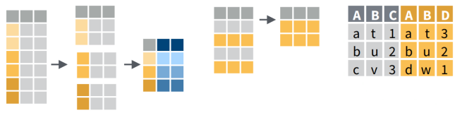
Joining Tables

Join tables on a common column

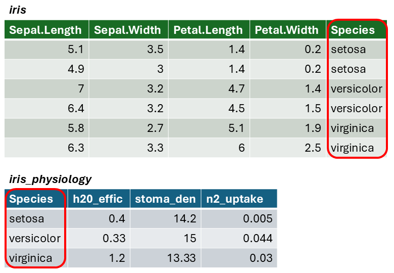
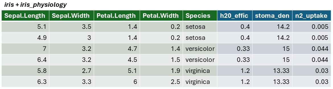
The result of a join is additional columns.

To join two data frames based on a common column, you can use:

left_join(x, y, by)

where x and y are data frames, and by is the name of a column they have in common.

Join columns must be the same data type (i.e., both numeric or both character).

If there is only one column in common, and if it has the same name in both data frames, you can omit the by argument.

The by argument can take the join_by() for more complex cases (e.g., join columns have different names)

Simple Join Example

To illustrate a table join, we'll first import a csv with some fake data about the genetics of different iris species:

# Create a data frame with additional info about the three IRIS species
iris_genetics <- data.frame(Species=c("setosa", "versicolor", "virginica"),
                          num_genes = c(42000, 41000, 43000),
                          prp_alles_recessive = c(0.8, 0.76, 0.65))

iris_genetics

##      Species num_genes prp_alles_recessive
## 1     setosa     42000                0.80
## 2 versicolor     41000                0.76
## 3  virginica     43000                0.65

We can join these additional columns to the iris data frame with left_join():

iris |> 
  left_join(iris_genetics, by = "Species") |> 
  slice(1:10)

##    Sepal.Length Sepal.Width Petal.Length Petal.Width Species num_genes
## 1           5.1         3.5          1.4         0.2  setosa     42000
## 2           4.9         3.0          1.4         0.2  setosa     42000
## 3           4.7         3.2          1.3         0.2  setosa     42000
## 4           4.6         3.1          1.5         0.2  setosa     42000
## 5           5.0         3.6          1.4         0.2  setosa     42000
## 6           5.4         3.9          1.7         0.4  setosa     42000
## 7           4.6         3.4          1.4         0.3  setosa     42000
## 8           5.0         3.4          1.5         0.2  setosa     42000
## 9           4.4         2.9          1.4         0.2  setosa     42000
## 10          4.9         3.1          1.5         0.1  setosa     42000
##    prp_alles_recessive
## 1                  0.8
## 2                  0.8
## 3                  0.8
## 4                  0.8
## 5                  0.8
## 6                  0.8
## 7                  0.8
## 8                  0.8
## 9                  0.8
## 10                 0.8

Data Wrangling with R Pt I

Start Recording

About Me...

IGIS Team

Some of My R Work

degday

uasimg

caladaptR

T-Locoh

Shiny Apps

About You...

Workshop Goals

Data Wrangling: What do we mean?

Operations

Outline

Planning Your Data Wrangling Strategy

What is "tidy data"?

Are these data 'tidy'?

Do I have to use tidy data?

Advantages of tidy data

Reasons not to use tidy data

Data Wrangling Methods

Tidyverse

Core Packages

Better Ways to Import Tabular Data

Explore Data

Structure

Preview the data

Distribution and Frequency

Plots

Missing Values

Little bit of everything

Data Wrangling with dplyr

Popular dplyr Functions

Row and Column Manipulations

Subset Rows

Chaining dplyr functions

Example

stringr

ggplot

Anatomy of a ggplot

Maping Columns to Symbology Properties with aes()

Geoms

Example:

Adding visual elements to a plot

Exercise 1

Break!

Highlights of Exercise 1

tidy-select Expressions

Data File Formats

Group and Summarize

Joining Tables

Join tables on a common column

Simple Join Example

Exercise 2

Data Wrangling with `dplyr`

Popular `dplyr` Functions

`stringr`

Maping Columns to Symbology Properties with `aes()`