Some of My R Work

degday

Compute degree days in R
https://ucanr-igis.github.io/degday/

uasimg

Data management utilities for drone mapping
https://ucanr-igis.github.io/uasimg/

caladaptR

Bring climate data from Cal-Adapt into R using the API
https://ucanr-igis.github.io/caladaptr/

T-Locoh

Homerange and spatial-temporal pattern analysis for wildlife tracking data
http://tlocoh.r-forge.r-project.org/

Shiny Apps

Chill Portions Under Climate Change Calculator
https://ucanr-igis.shinyapps.io/chill/

Drone Mission Planner for Reforestation Monitoring Protocol
https://ucanr-igis.shinyapps.io/uav_stocking_survey/

Stock Pond Volume Calculator
https://ucanr-igis.shinyapps.io/PondCalc/

Pistachio Nut Growth Calculator
https://ucanr-igis.shinyapps.io/pist_gdd/

Data Wrangling: What do we mean?

Whatever is needed to get your data frame ready
for the function(s) you want to use for analysis and visualization.

Also called: data munging, data manipulation, data transformation, etc.

Operations

Data wrangling often includes some combination of:

dropping columns
renaming columns
changing the order of columns
creating new columns with an expression
filtering rows
sorting rows
going from ‘long’ to ‘wide’ formats
joining data frames based on a common field
merging / stacking data frames together
splitting tables
aggregating rows into groups
splitting columns into new columns / rows

Outline

Developing a strategy

What is tidy data?
Working backwards

R Methods

Functions and piping
Importing data
Subsetting rows and columns
Creating new columns
Type conversions: text, dates, numbers, units
Reshaping data
Dealing with missing values
Joinging tables
Grouping and summarizing rows

More advanced tasks

Wrangling really large data
Flattening nested data
Splitting flat data into relational tables
Reading and writing databases
??

But wait.

Can’t ChatGPT just take
care of this
for me?

Learning with GenAI

https://www.tidyverse.org/blog/2025/04/learn-tidyverse-ai/

Highlights

ChatGPT will give you code.
It may or may not work.
It may or may not be good code (probably not).
You should always cross check it with the documentation.

Suggestions for Using ChatGPT to Learn Data Wrangling

“Use code completion tools sparingly if you’re a new user.”
ChatGPT is good for getting starter code, discovering functions, arguments, solving a simple, well-defined problem, etc.
Break a task into smaller steps.
Don’t depend on ChatGPT to create a workflow or chain
Be wary of code you don’t understand.
R has great documentation & tutorials online - take advantage of it.

Planning Your Data Wrangling Strategy

What is “tidy data”?

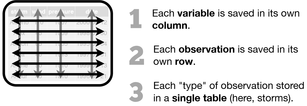
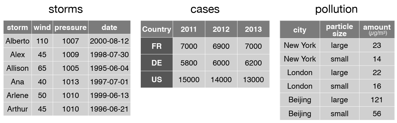
R functions like tidy data!

Are these data ‘tidy’?

Functions

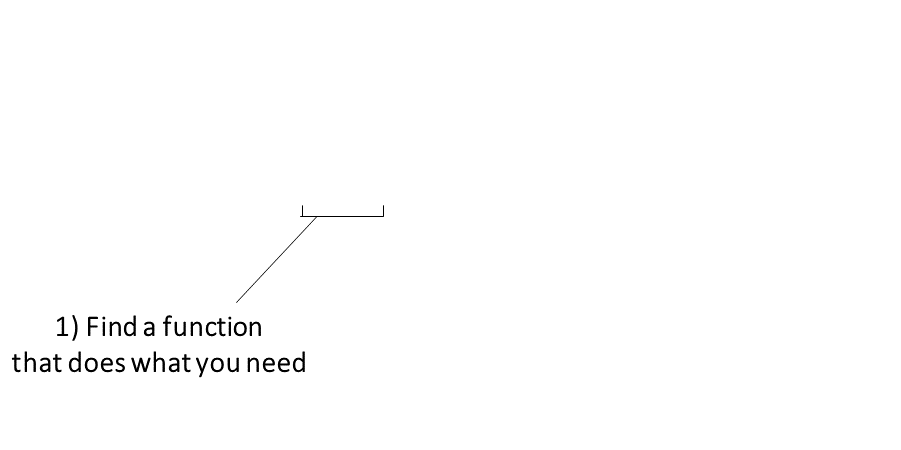
The keys to R’s superpowers are functions! There are four things you need to know to use a function:

What Do Functions Return?

numbers
dates
text
data frames and matrices
spatial data
plots
trained regression models
HTML widgets
another function that returns a color ramp
a drone image collection metadata record
⇒ almost anything you can think of can be returned by a function!!
⇒ anything returned by a function can also be saved to an object

Which function should I use?

Finding the right R function, half the battle is.

- Jedi MasteR Yoda

Ask your friends

Ask Google / ChatGPT

Cheatsheets!

Function Help

Every function has a help page. To get to it enter ? followed by the name of the function (without parentheses):

?rnorm

Function Arguments

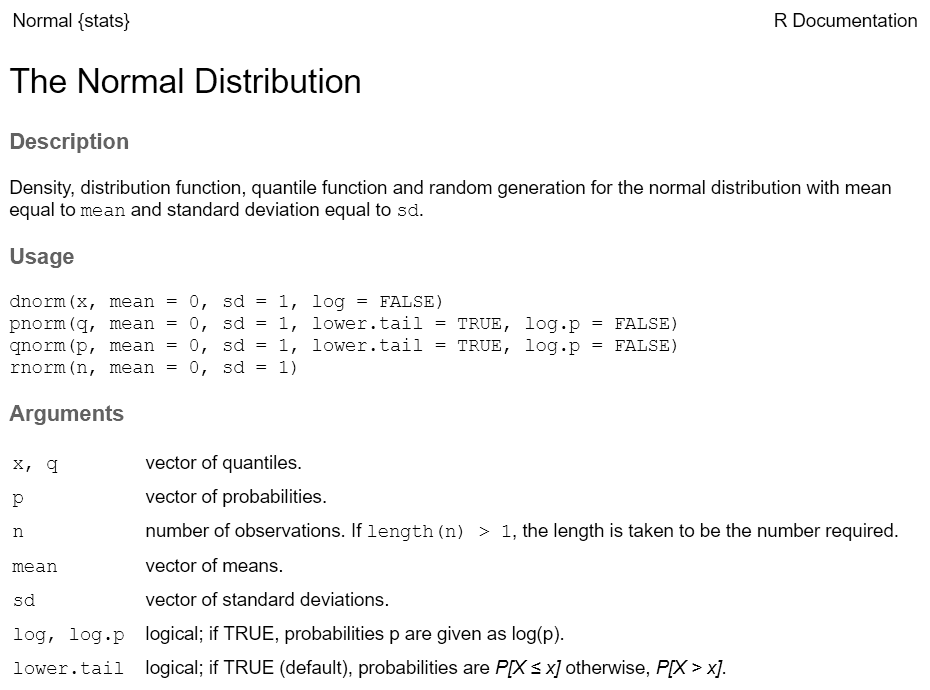
Most functions take arguments. Arguments can be required or optional (i.e. have a default value).

See the function’s help page to determine which arguments are expected. Example:

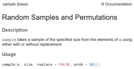
x and size have no default value → they are required

replace and prob have default values → they are optional

To name or not to name your arguments? That is the question.

All arguments have names. You can explicitly name arguments when calling a function as follows:

rnorm(n = 100, mean = 10, sd = 0.3)

Benefits of naming your arguments:

Helps you remember what each argument is
You can enter then in any order
You can skip arguments if you’re happy with the default value

But you can omit argument names if you pass them in the order expected and don’t skip any.

rnorm(500, 50, 3)  ## generate 500 normally distributed random
                   ## numbers with a mean of 50 and stand dev = 3.

Piping

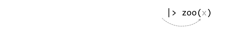
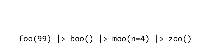
Piping syntax is an alternative way of writing arguments into functions.

With piping, you use the pipe operator |> (or %>%) to ‘feed’ the result of one function into the next function.

Piping allows the results of one function to be passed as the first argument of the next function. Hence a series of commands to be written like a sentence.

Example

Consider the expression:

zoo(moo(boo(foo(99)),n=4))

Piping Tips and Tricks

Keyboard shortcut for inserting the pipe operator: ctrl + shift + m

You can tell RStudio which pipe to insert under Global Options >> Code

|> (‘native’ pipe introduced R4.0)

%>% (from magrittr package)

To split a chain of functions across multiple lines, end each line with a pipe operator:

seq(1, 10, 0.1) |> 
  log() |> 
  sum()

## [1] 141.4023

If the receiving function requires additional arguments, just add them starting with the 2nd argument (or use named arguments):

runif(5) |> round(2)

## [1] 0.99 0.69 0.76 0.88 0.55

Same Function Name, Different Packages

Occasionally two or more packages will have different functions that use the same name.

When this happens, R will use whichever one was loaded first.

Best practice: use the package name and the :: reference to specify which package a function is from.

x <- sp::over()
x <- grDevices::over()

y <- raster::select()
y <- dplyr::select()

When you use the package_name::function_name syntax, you don’t actually have to first load the package with library().

Resolving Name Conflicts with the conflicted Package

When you call a function that exists in multiple packages, R uses whichever package was loaded first.

The conflicted package helps you avoid problems with duplicate function names, by specifying which one to prioritize no matter what order they were loaded.

library(conflicted)

# Set conflict preference
conflict_prefer("filter", "dplyr")
conflict_prefer("count", "dplyr")
conflict_prefer("select", "dplyr")

# From here on out, anytime we call select() or filter(), R will
# always use the dplyr version.

Data Wrangling Methods

Better Ways to Import Tabular Data

These packages allow you to:

import tabular data in different formats
skip rows that don’t actually contain data
specify whether the file contains a header
rename columns as part of the importing
specify the data type for each column

Example:

library(readxl)
my_tbl = read_xlsx(path = "plot_data.xlsx", 
                   sheet = "Sheet2",
                   skip = 3,
                   col_names = c("plot_num", "date", "species", "count"),
                   col_types = c("text", "date", "text", "integer"))

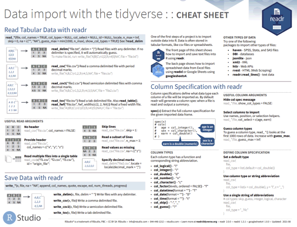
Data Wrangling with `dplyr`

An alternative (usually better) way to wrangle data frames than base R.

Part of the tidyverse.

Best way to familiarize yourself - explore the cheat sheet:

Popular `dplyr` Functions

Row and Column Manipulations

subset rows	filter(), slice()
order rows	arrange()
pick column(s)	select(), pull()
add new columns	mutate()

Chaining dplyr functions

Most dplyr functions take a tibble as the first argument , and return a tibble.

This makes them very pipe friendly.

Example

Look at the storms tibble:

library(dplyr)
head(storms)

## # A tibble: 6 × 13
##   name   year month   day  hour   lat  long status       category  wind pressure
##   <chr> <dbl> <dbl> <int> <dbl> <dbl> <dbl> <fct>           <dbl> <int>    <int>
## 1 Amy    1975     6    27     0  27.5 -79   tropical de…       NA    25     1013
## 2 Amy    1975     6    27     6  28.5 -79   tropical de…       NA    25     1013
## 3 Amy    1975     6    27    12  29.5 -79   tropical de…       NA    25     1013
## 4 Amy    1975     6    27    18  30.5 -79   tropical de…       NA    25     1013
## 5 Amy    1975     6    28     0  31.5 -78.8 tropical de…       NA    25     1012
## 6 Amy    1975     6    28     6  32.4 -78.7 tropical de…       NA    25     1012
## # ℹ 2 more variables: tropicalstorm_force_diameter <int>,
## #   hurricane_force_diameter <int>

Filter out only the records for category 3 or higher storms

storms |> 
  select(name, year, month, category) |>     ## select the columns we need
  filter(category >= 3)                      ## select just the rows we want

## # A tibble: 1,262 × 4
##    name      year month category
##    <chr>    <dbl> <dbl>    <dbl>
##  1 Caroline  1975     8        3
##  2 Caroline  1975     8        3
##  3 Eloise    1975     9        3
##  4 Eloise    1975     9        3
##  5 Gladys    1975    10        3
##  6 Gladys    1975    10        3
##  7 Gladys    1975    10        4
##  8 Gladys    1975    10        4
##  9 Gladys    1975    10        3
## 10 Belle     1976     8        3
## # ℹ 1,252 more rows

dplyr functions generally allow you to enter column names without quotes.

Palmer Penguins

The Palmer Penguins dataset contains field data for three species of penguins.

Exercise 1

In this exercise, we will:

Import some messy data from Excel
Wrangle the Penguins!

Subset columns
Compute new columns
Sort and subset rows

This exercise will be done in an R Notebook!

https://posit.cloud/content/10255792

`dplyr` Pro Tips

Advanced `select()`

select(-age)	Select all columns except age
select(fname:grade)	Select all columns between `fname` and `grade`
select(starts_with(“Sepal”))	Select all columns that start with ‘Sepal’ (see also `ends_width()`, `contains()`, and `matches()`

Renaming columns

my_dataframe |> rename(fname = First, lname = Last)
my_dataframe |> select(fname = First, lname = Last, term, grade,
passed)

Joining Tables

`dplyr` join functions

join data frames on a column	left_join(), right_join(), inner_join()
stack data frames	bind_rows()

Join tables on a common column

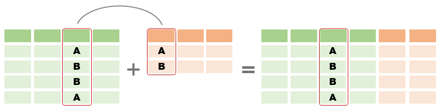
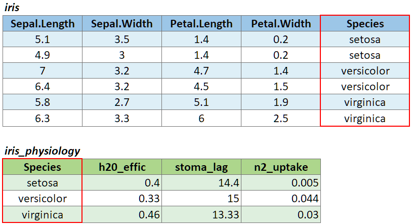
To join two data frames based on a common column, you can use:

left_join(x, y, by)

where x and y are data frames, and by is the name of a column they have in common.

If there is only one column in common, and if it has the same name in both data frames, you can omit the by argument.

If the common column is named differently in the two data frames, you can deal with that by passing a named vector as the by argument. See below.

To illustrate a table join, we’ll first import a csv with some fake data about the genetics of different iris species:

# Create a data frame with additional info about the three IRIS species
iris_genetics <- data.frame(Species=c("setosa", "versicolor", "virginica"),
                          num_genes = c(42000, 41000, 43000),
                          prp_alles_recessive = c(0.8, 0.76, 0.65))

iris_genetics

##      Species num_genes prp_alles_recessive
## 1     setosa     42000                0.80
## 2 versicolor     41000                0.76
## 3  virginica     43000                0.65

We can join these additional columns to the iris data frame with left_join():

iris |> 
  left_join(iris_genetics, by = "Species") |> 
  slice(1:10)

##    Sepal.Length Sepal.Width Petal.Length Petal.Width Species num_genes
## 1           5.1         3.5          1.4         0.2  setosa     42000
## 2           4.9         3.0          1.4         0.2  setosa     42000
## 3           4.7         3.2          1.3         0.2  setosa     42000
## 4           4.6         3.1          1.5         0.2  setosa     42000
## 5           5.0         3.6          1.4         0.2  setosa     42000
## 6           5.4         3.9          1.7         0.4  setosa     42000
## 7           4.6         3.4          1.4         0.3  setosa     42000
## 8           5.0         3.4          1.5         0.2  setosa     42000
## 9           4.4         2.9          1.4         0.2  setosa     42000
## 10          4.9         3.1          1.5         0.1  setosa     42000
##    prp_alles_recessive
## 1                  0.8
## 2                  0.8
## 3                  0.8
## 4                  0.8
## 5                  0.8
## 6                  0.8
## 7                  0.8
## 8                  0.8
## 9                  0.8
## 10                 0.8

If you need to join tables on multiple columns, add additional column names to the by argument.

Join columns must be the same data type (i.e., both numeric or both character).

There are several variants of left_join(), the most common being right_join() and inner_join(). See help for details.

Joining Tables When the Column Name is Different

If the join column is named differently in the two tables, you can pass a named character vector as the by argument. A named vector is a vector whose elements have been assigned names. You can construct a named vector with c().

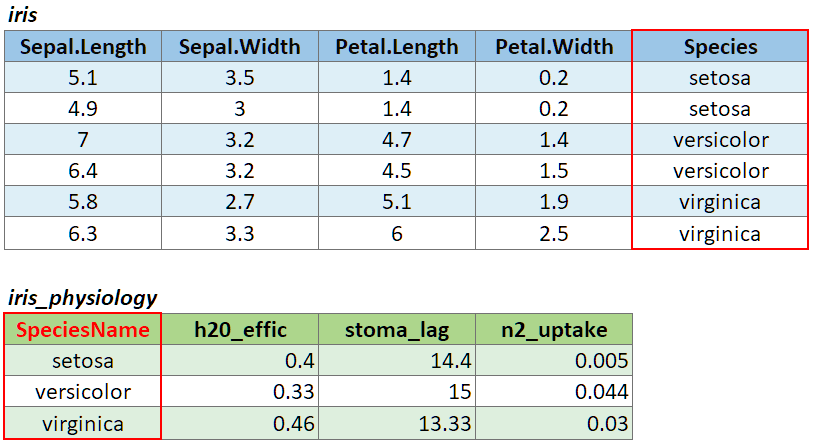
For example if the join column was named ‘SpeciesName’ in x, and just ‘Species’ in y, your expression would be:

left_join(x, y, by = c("SpeciesName" = "Species"))

Stacking or Merging Data Frames

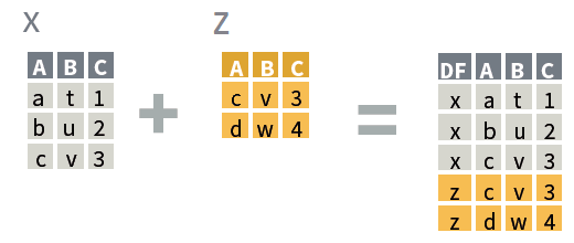
bind_rows(x, y)

where x and y:

are data frames
have the exact same column structure (names, order, & class)
you can add more than two data frames

Reshaping Data

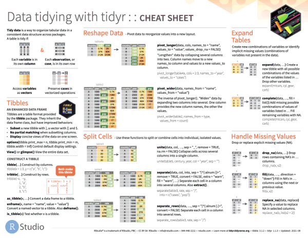
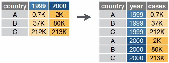
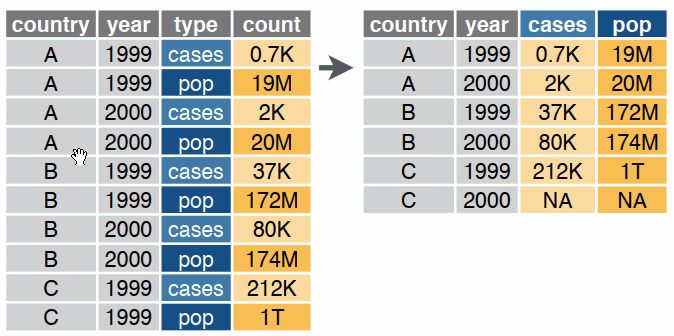
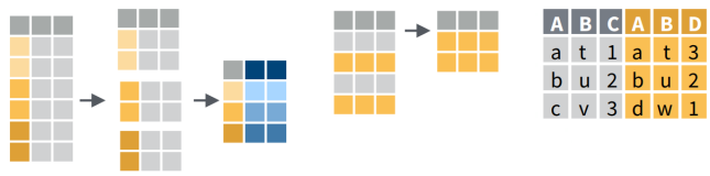
Reshaping data includes:

turning rows into columns (aka pivot tables, cross tab query)
turning columns into rows

The go-to Tidyverse package for reshaping data frames is tidyr

Pivot Functions

pivot_longer()

pivot_wider()

More info and examples in the tidyr Pivoting Vignette

Group and Summarize

Step 1 (optional): group rows (i.e., change the unit of analysis)	`group_by()`
Step 2: Compute summaries for each group of rows	Add summary columns with `summarize()` Aggregate functions available: `n(), mean(), median(), sum(), sd(), IQR(), first(),` etc.

Example:

library(dplyr)
head(storms)

## # A tibble: 6 × 13
##   name   year month   day  hour   lat  long status       category  wind pressure
##   <chr> <dbl> <dbl> <int> <dbl> <dbl> <dbl> <fct>           <dbl> <int>    <int>
## 1 Amy    1975     6    27     0  27.5 -79   tropical de…       NA    25     1013
## 2 Amy    1975     6    27     6  28.5 -79   tropical de…       NA    25     1013
## 3 Amy    1975     6    27    12  29.5 -79   tropical de…       NA    25     1013
## 4 Amy    1975     6    27    18  30.5 -79   tropical de…       NA    25     1013
## 5 Amy    1975     6    28     0  31.5 -78.8 tropical de…       NA    25     1012
## 6 Amy    1975     6    28     6  32.4 -78.7 tropical de…       NA    25     1012
## # ℹ 2 more variables: tropicalstorm_force_diameter <int>,
## #   hurricane_force_diameter <int>

For each month, how many storm observations are saved in the data frame

storms |> 
  select(name, year, month, category) |>    ## select the columns we need
  group_by(month) |>                        ## group the rows by month
  summarize(num_storms = n())               ## for each group, report the count

## # A tibble: 10 × 2
##    month num_storms
##    <dbl>      <int>
##  1     1         70
##  2     4         66
##  3     5        201
##  4     6        809
##  5     7       1651
##  6     8       4442
##  7     9       7778
##  8    10       3138
##  9    11       1170
## 10    12        212

Data Wrangling with R

Start Recording

About Me…

IGIS Team

Some of My R Work

degday

uasimg

caladaptR

T-Locoh

Shiny Apps

About You…

Data Wrangling: What do we mean?

Operations

Tools of the Trade

Tools of the Trade

Outline

But wait. Can’t ChatGPT just takecare of this for me?

Learning with GenAI

Planning Your Data Wrangling Strategy

What is “tidy data”?

Are these data ‘tidy’?

R Fundamentals

Functions

What Do Functions Return?

Which function should I use?

Function Help

Function Arguments

To name or not to name your arguments? That is the question.

Piping

Example

Piping Tips and Tricks

Same Function Name, Different Packages

Data Wrangling Methods

Better Ways to Import Tabular Data

Data Wrangling with dplyr

Popular dplyr Functions

Row and Column Manipulations

Chaining dplyr functions

Example

Palmer Penguins

Exercise 1

Break!

dplyr Pro Tips

Advanced select()

Renaming columns

Joining Tables

dplyr join functions

Join tables on a common column

Joining Tables When the Column Name is Different

Stacking or Merging Data Frames

Reshaping Data

Pivot Functions

Group and Summarize

Notebook Exercise #2

But wait.

Can’t ChatGPT just take
care of this
for me?

Data Wrangling with `dplyr`

Popular `dplyr` Functions

`dplyr` Pro Tips

Advanced `select()`

`dplyr` join functions