Intro to R Part 2:
Packages, Functions, Data Frames,
and
Importing Data

Andy
Lyons
October 12, 2022
https://ucanr-igis.github.io/IntroR_Oct22/


Review from Part I
R as a fancy calculator:
(pi
* 5 ^ 2) / sqrt(4 / 3)
Saving results as objects:
my_volume = (4 / 3) * pi * (1.5 ^ 3)
All R objects have a class (e.g., numeric, character,
data frame)
Objects that contain multiple values of the same class are called
vectors
Some functions that return
vectors:
seq()
rnorm()
sample()
You can build vectors from scratch using:
c()
You can subset or extract elements from vectors using square
brackets:
With a
vector of integers (indices):
LETTERS[1:4]
Logical vector:
LETTERS[
c(T,T,T,T,F,F,F,F,F,F,F,F,F,F,F,F,F,F,F,F,F,F,F,F,F,F)
]
Logical expression:
x =
1:100
x [x %% 3 == 0]
Functions and operators that do something to each element of a
vector and return another vector are said to be
vectorized
+ - * /
round(), abs()
Functions that take multiple elements of a vector and spit out a
single value are said to be aggregate
functions
sum(), min(), mean(), max()
R comes with some basic plot functions:
hist(x)
boxplot(x)
plot(x, y) ## scatterplot
plot(x, y, type = 'b') ## 'b' = plot both points and lines
Warm-Up Quiz

Today’s Outline
First half
- packages
- functions
- piping syntax
- Exercise 3
Second half
- data frames
- importing CSV files
- Exercise 4
R Packages

Packages are what R calls extensions or
add-ons.
What’s in a package?
- additional functions!
- function help pages
- tutorials (Vignettes)
- datasets
Installing and Using Packages
Three simple steps to use the functions in a package:
Figure out which package you need
Install (i.e., download) it (just once)
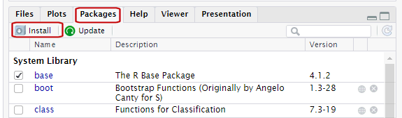
- Load it into memory (must do this every time you start
RStudio)
Functions
The keys to R’s superpowers are functions! There are
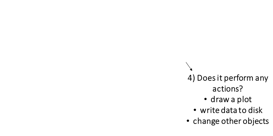
four things you need to know to use a function:
What Do Functions Return?
- numbers
- dates
- text
- data frames and matrices
- spatial data
- plots
- trained regression models
- HTML widgets
- another function that returns a color ramp
- a drone image collection metadata record
- ⇒ almost anything you can think of can
be returned by a function!!
- ⇒ anything returned by a function can
also be saved to an object
Which function should I use?
Finding the right R function, half the battle is.
- Jedi MasteR
Yoda
|

|
Ask your friends
Ask Google
Cheatsheets!
Function Help
Every function has a help page. To get to it enter ?
followed by the name of the function (without parentheses):
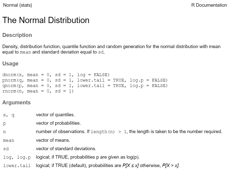
Function Arguments
Most functions take arguments. Arguments can be required or
optional (i.e. have a default value).
See the function’s help page to determine which arguments are
expected. Example:
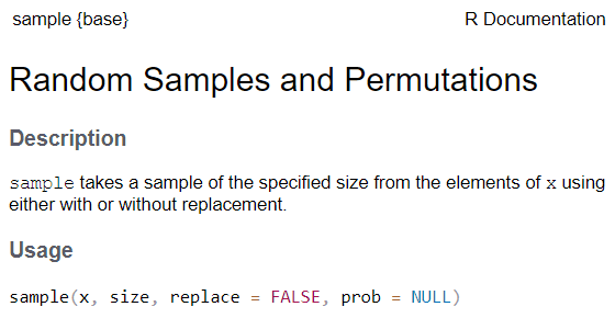
x and size have no default value → they are
required
replace and prob have default values → they
are optional
To
name or not to name your arguments? That is the question.
All arguments have names. You can explicitly name arguments when
calling a function as follows:
rnorm(n = 100, mean = 10, sd = 0.3)
Benefits of naming your arguments:
- Helps you remember what each argument is
- You can enter then in any order
- You can skip arguments if you’re happy with the default value
But you can omit argument names if you pass them in
the order expected and don’t skip any.
rnorm(500, 50, 3)  ## generate 500 normally distributed random
                   ## numbers with a mean of 50 and stand dev = 3.
Piping

Piping syntax is an alternative way of writing
arguments into functions.
With piping, you use the pipe operator %>% or |> to ‘feed’ the result of one function
into the next function.
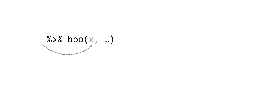
Piping allows the results of one function to be passed as the
first argument of the next function. Hence a series of
commands to be written like a sentence.
Example
Consider the expression:
Piping Tips and Tricks
The traditional pipe character requires the magrittr or
dplyr package.
Keyboard shortcut for inserting the pipe operator:
ctrl + shift + m
You can tell RStudio which pipe to insert under Global Options
>> Code
%>% (traditional,
default)
|> (‘native’ pipe
introduced R4.0)
To split a chain of functions across multiple lines, end
each line with a pipe operator:
seq(1, 10, 0.1) %>%
  log() %>%
  sum()
## [1] 141.4023
If the receiving function requires additional arguments, just add
them starting with the 2nd argument (or use named
arguments):
## [1] 0.07 0.71 0.06 0.08 0.48
Need to pipe to an argument that isn’t the first? Indicate
where pipe values should go with a dot:
## gsub() does find-replace on character values:
c("apple", "banana", "pear") %>% gsub("a", "-", .)
## [1] "-pple" "b-n-n-" "pe-r"
Exercise 3: Packages and Piping
Exercise 3 Topics
- Installing packages
- Loading packages into memory with
library()
- Piping syntax
Break!
Data Frames
R has two data classes that organize data in rows and columns:
Rows and Columns by any
other name….
rows
aka:
- record
- case
- feature (spatial)
columns
aka: variable, field
##   Sepal.Length Sepal.Width Petal.Length Petal.Width Species
## 1          5.1         3.5          1.4         0.2  setosa
## 2          4.9         3.0          1.4         0.2  setosa
## 3          4.7         3.2          1.3         0.2  setosa
## 4          4.6         3.1          1.5         0.2  setosa
## 5          5.0         3.6          1.4         0.2  setosa
## 6          5.4         3.9          1.7         0.4  setosa
Key concepts
- columns of a data frame are vectors
- columns have names
- you can refer to columns by their name or
position
Pulling out a Single Column
To get an individual column, use $
##   Girth Height Volume
## 1   8.3     70   10.3
## 2   8.6     65   10.3
## 3   8.8     63   10.2
## 4  10.5     72   16.4
## 5  10.7     81   18.8
## 6  10.8     83   19.7
##  [1] 70 65 63 72 81 83 66 75 80 75 79 76 76 69 75 74 85 86 71 64 78 80 74 72 77
## [26] 81 82 80 80 80 87
trees$Height %>% summary()
##    Min. 1st Qu.  Median    Mean 3rd Qu.    Max.
##      63      72      76      76      80      87
Subsetting rows and columns
You can use square bracket notation or tidyverse methods (dplyr).
Come back for Part 3. Data Wrangling
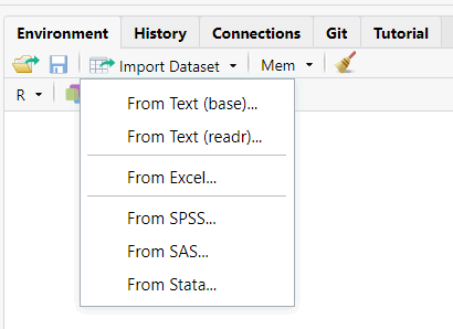
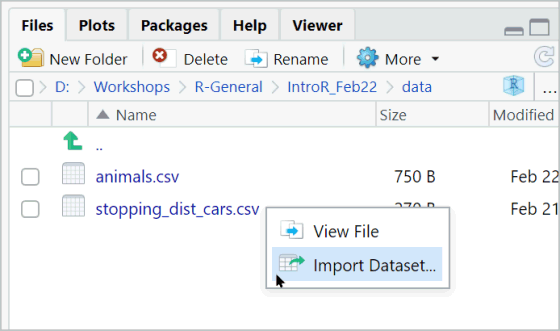
Importing Data: RStudio’s Import Dataset Wizard
File Paths
When you import (or export) data with code, you have to provide a
path to a file.
Paths can be absolute (full), or relative
working directory.
Complete path:
my_data = read.csv("C:/Users/Andy/Documents/LREC/n2_study/plots/plot34a/data/soil_moist.csv")
Windows users: Beware the slashes!
The following will not work beause of the slashes:
C:\noworm\trials\data
Back slashes must be converted to one of the following:
C:/noworm/trials/data
C:\\noworm\\trials\\data
Using Paths Relative to the Working Directory
Working Directory
Even though you don’t see it, there is always
working directory.
You can view the current working directory with:
Changing the working directory is easy!
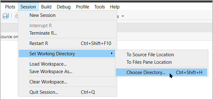
…or with code:
setwd("D:/Data/DroneData/black_rascal_creek")
Relative Paths
When using relative paths, the first '.' represents the
working directory.
my_data = read.csv("./data/soil_moist.csv")
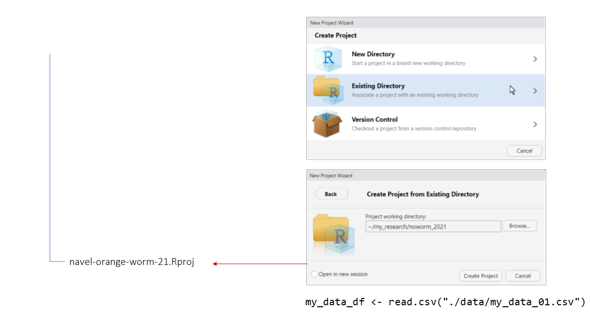
The main advantage of using relative paths is portability of
your project.
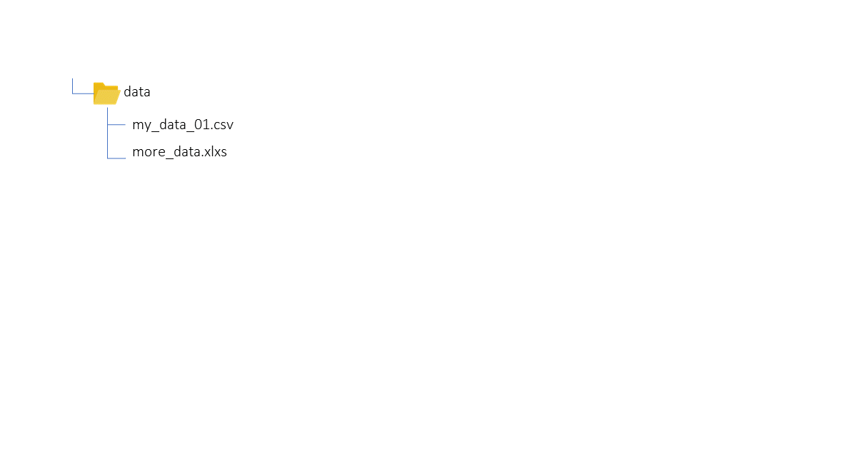
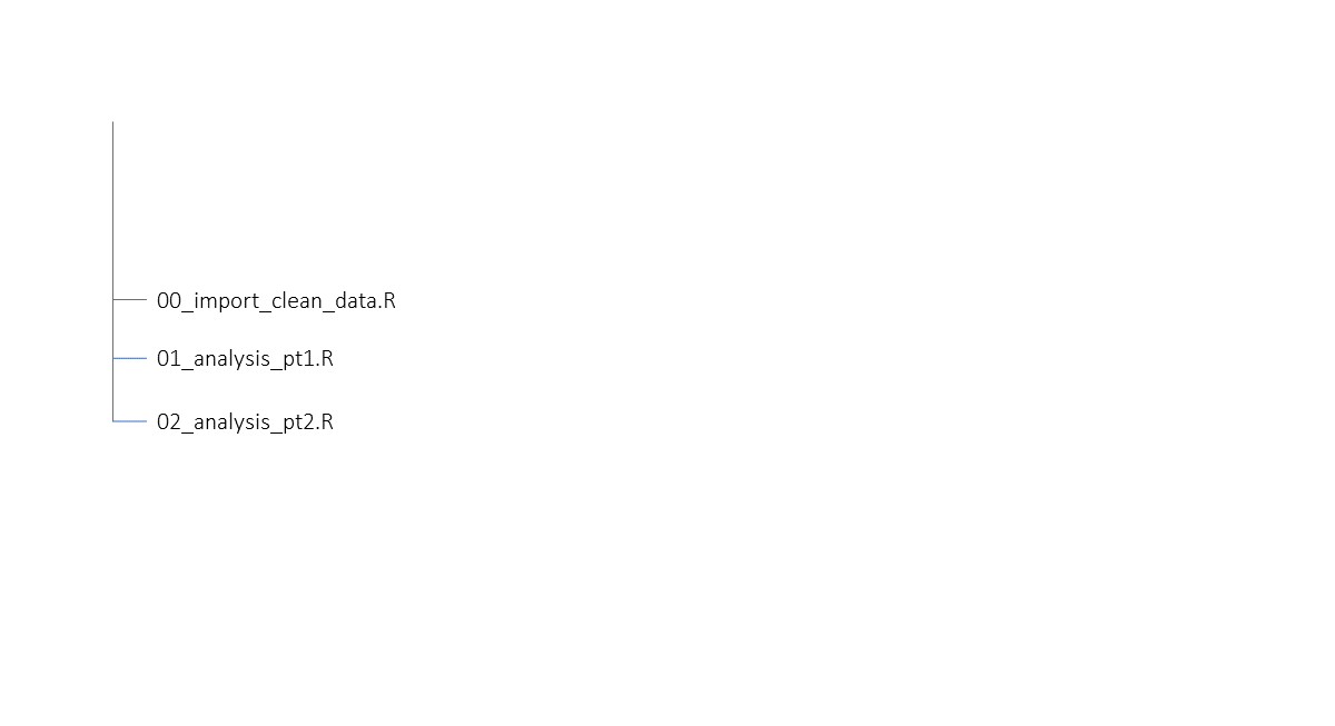
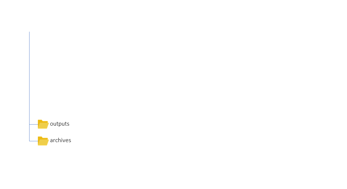
Organizing Data and Scripts
Exercise 4: Importing Data and Working with Data Frames
Exercise 4 Topics
- create data frames from scratch
- explore R’s built-in data frames
- compute summary stats on individual columns
- import a csv
- subset rows
- identify NA values
Review: Data Frames
The most common class for storing tabular data in R is the
data frame
View the first few rows of a data frame with
head()
View an entire data frame with
View()
Grab an individual column with $
END!