Review from Part II

Plotting

“Base R” comes with some basic plot functions:

hist(x)
boxplot(x)
plot(x, y) ## scatterplot
plot(x, y, type = 'b') ## 'b' = plot both points and lines

There are packages designing specifically for plotting (e.g., ggplot2)

Packages

packages are the key to productivity with R

packages mainly provide additional functions (and sometimes data)

the tidyverse is a family of packages for working with data

you can install packages from the ‘Packages’ pane in RStudio, or install.packages()

load packages into memory with library()

Functions

Piping Syntax

fun_a() |> fun_b() |> fun_c() |> …

iris |> filter(Sepal.Length > 7) |> mutate(width_length = Sepal.Width * Sepal.Length)
  │        │                             │
  │        │                             └─ create a new column
  │        │
  │        ├─ select those rows where Sepal.Length > 7
  │        └─ don't have to specify the data frame
  │    
  └ start with this data frame

Data Frames

The most common class for storing tabular data in R is the data frame

View the first few rows of a data frame with head()

View an entire data frame with View()

Grab an individual column with $

Importing Data

Base R function for importing csv files: read.csv()

RStudio also has an import dataset wizard

Packages available for importing specific file formats (e.g., SPSS)

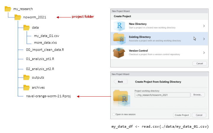
Paths to files can be absolute or relative (to the working directory)

Best practice for reproducibility and portability: RStudio projects

Don’t Forget Cheatsheets!

Data Wrangling: What do we mean?

Whatever is needed to get your data frame ready
for the function(s) you want to use for analysis and visualization.

also called data munging, manipulation, transformation, etc.

Often includes one or more of:

dropping columns
renaming columns
changing the order of columns
creating new columns with an expression
filtering rows
sorting rows
going from ‘long’ to ‘wide’ formats
joining data frames based on a common field
merging data frames together
splitting tables
aggregating rows into groups

What is “tidy data”?

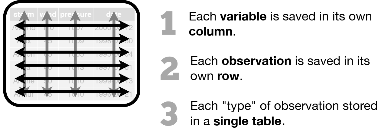
R functions like tidy data!

Are these data ‘tidy’?

Better Ways to Import Data

The functions in these packages allow you to:

import tables from different formats
skip rows that don’t actually contain data
skip lines that start with a comment character
specify whether the file contains a header
rename columns as part of the importing
specify the data type for each column

Example:

library(readxl)
my_tbl = read_xlsx(path = "plot_data.xlsx", 
                   sheet = "Sheet2",
                   skip = 3,
                   col_names = c("plot_num", "date", "species", "count"),
                   col_types = c("text", "date", "text", "integer"))

Data Wrangling with `dplyr`

An alternative (usually better) way to wrangle data frames than base R.

Part of the tidyverse.

Best way to familiarize yourself - explore the cheat sheet:

Popular `dplyr` Functions

Row and Column Manipulations

subset rows	filter(), slice()
order rows	arrange()
pick column(s)	select(), pull()
add new columns	mutate()

Chaining dplyr functions

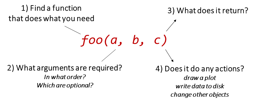
Most dplyr functions take a tibble as the first argument , and return a tibble.

This makes them very pipe friendly.

Example

Look at the storms tibble:

library(dplyr)
head(storms)

## # A tibble: 6 × 13
##   name   year month   day  hour   lat  long status       category  wind pressure
##   <chr> <dbl> <dbl> <int> <dbl> <dbl> <dbl> <fct>           <dbl> <int>    <int>
## 1 Amy    1975     6    27     0  27.5 -79   tropical de…       NA    25     1013
## 2 Amy    1975     6    27     6  28.5 -79   tropical de…       NA    25     1013
## 3 Amy    1975     6    27    12  29.5 -79   tropical de…       NA    25     1013
## 4 Amy    1975     6    27    18  30.5 -79   tropical de…       NA    25     1013
## 5 Amy    1975     6    28     0  31.5 -78.8 tropical de…       NA    25     1012
## 6 Amy    1975     6    28     6  32.4 -78.7 tropical de…       NA    25     1012
## # ℹ 2 more variables: tropicalstorm_force_diameter <int>,
## #   hurricane_force_diameter <int>

Filter out only the records for category 3 or higher storms

storms |> 
  select(name, year, month, category) |>     ## select the columns we need
  filter(category >= 3)

## # A tibble: 1,233 × 4
##    name      year month category
##    <chr>    <dbl> <dbl>    <dbl>
##  1 Caroline  1975     8        3
##  2 Caroline  1975     8        3
##  3 Eloise    1975     9        3
##  4 Eloise    1975     9        3
##  5 Gladys    1975    10        3
##  6 Gladys    1975    10        3
##  7 Gladys    1975    10        4
##  8 Gladys    1975    10        4
##  9 Gladys    1975    10        3
## 10 Belle     1976     8        3
## # ℹ 1,223 more rows

Observe that with dplyr functions you generally don’t have to put column names in quotes

Many more examples in the exercise!

Duplicate Function Names

Occasionally two or more packages will have a function with the same name.

R will use whichever one was loaded first.

Best practice: use the package name and the :: reference to specify which package a function is from.

x <- sp::over()
x <- grDevices::over()

y <- raster::select()
y <- dplyr::select()

When you use the package_name::function_name syntax, you don’t actually have to first load the package with library().

Resolving Name Conflicts with the conflicted Package

When you call a function that exists in multiple packages, R uses whichever package was loaded first.

The conflicted package helps you avoid problems with duplicate function names, by specifying which one to prioritize no matter what order they were loaded.

library(conflicted)

# Set conflict preference
conflict_prefer("filter", "dplyr")
conflict_prefer("count", "dplyr")
conflict_prefer("select", "dplyr")

# From here on out, anytime we call select() or filter(), R will
# always use the dplyr version.

R Notebooks

R Notebooks are written in “R Markdown”, which combines text and R code.

Notebook Exercise: Wrangle the Penguins

Data

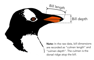
We’ll be looking at the Palmer Penguins dataset.

This exercise will be R Notebook!

Importing messy data from Excel
Subsetting columns
Calculating columns
Sorting and subsetting rows

Pro Tips

Renaming columns

my_dataframe |> rename(fname = First, lname = Last)
my_dataframe |> select(fname = First, lname = Last, term, grade,
passed)

Advanced `select()`

select(-age)	Select all columns except age
select(fname:grade)	Select all columns between `fname` and `grade`
select(starts_with(“Sepal”))	Select all columns that start with ‘Sepal’ (see also `ends_width()`, `contains()`, and `matches()`

Joining and Merging Tables

join data frames on a column	left_join(), right_join(), inner_join()
stack data frames	bind_rows()

Join tables on a common column

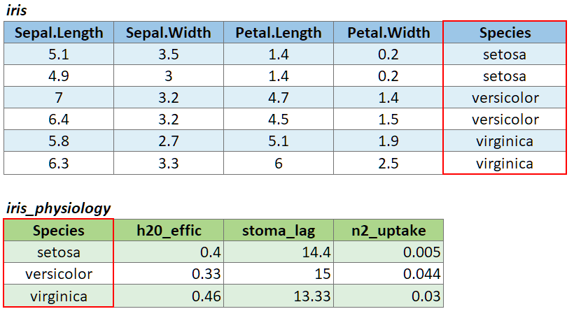
To join two data frames based on a common column, you can use:

left_join(x, y, by)

where x and y are data frames, and by is the name of a column they have in common.

If there is only one column in common, and if it has the same name in both data frames, you can omit the by argument.

If the common column is named differently in the two data frames, you can deal with that by passing a named vector as the by argument. See below.

To illustrate a table join, we’ll first import a csv with some fake data about the genetics of different iris species:

# Create a data frame with additional info about the three IRIS species
iris_genetics <- data.frame(Species=c("setosa", "versicolor", "virginica"),
                          num_genes = c(42000, 41000, 43000),
                          prp_alles_recessive = c(0.8, 0.76, 0.65))

iris_genetics

##      Species num_genes prp_alles_recessive
## 1     setosa     42000                0.80
## 2 versicolor     41000                0.76
## 3  virginica     43000                0.65

We can join these additional columns to the iris data frame with left_join():

iris |> 
  left_join(iris_genetics, by = "Species") |> 
  slice(1:10)

##    Sepal.Length Sepal.Width Petal.Length Petal.Width Species num_genes
## 1           5.1         3.5          1.4         0.2  setosa     42000
## 2           4.9         3.0          1.4         0.2  setosa     42000
## 3           4.7         3.2          1.3         0.2  setosa     42000
## 4           4.6         3.1          1.5         0.2  setosa     42000
## 5           5.0         3.6          1.4         0.2  setosa     42000
## 6           5.4         3.9          1.7         0.4  setosa     42000
## 7           4.6         3.4          1.4         0.3  setosa     42000
## 8           5.0         3.4          1.5         0.2  setosa     42000
## 9           4.4         2.9          1.4         0.2  setosa     42000
## 10          4.9         3.1          1.5         0.1  setosa     42000
##    prp_alles_recessive
## 1                  0.8
## 2                  0.8
## 3                  0.8
## 4                  0.8
## 5                  0.8
## 6                  0.8
## 7                  0.8
## 8                  0.8
## 9                  0.8
## 10                 0.8

If you need to join tables on multiple columns, add additional column names to the by argument.

Join columns must be the same data type (i.e., both numeric or both character).

There are several variants of left_join(), the most common being right_join() and inner_join(). See help for details.

Joining Tables When the Column Name is Different

If the join column is named differently in the two tables, you can pass a named character vector as the by argument. A named vector is a vector whose elements have been assigned names. You can construct a named vector with c().

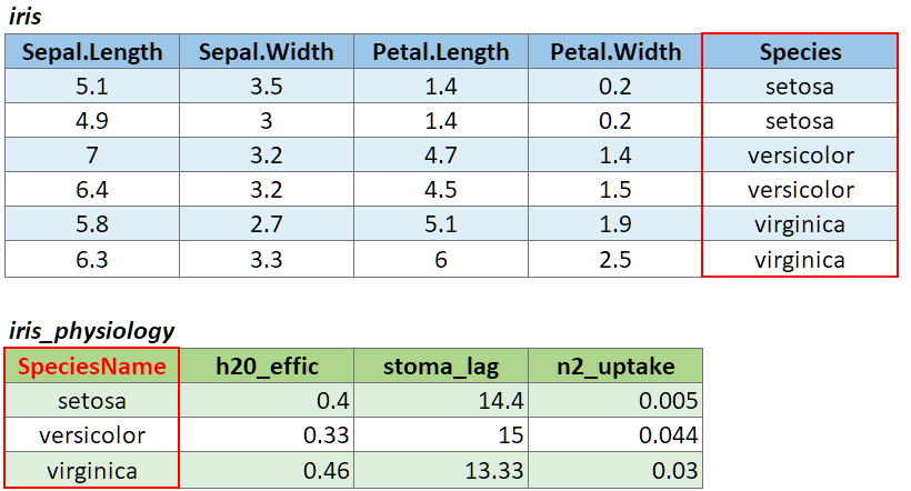
For example if the join column was named ‘SpeciesName’ in x, and just ‘Species’ in y, your expression would be:

left_join(x, y, by = c("SpeciesName" = "Species"))

Stacking or Merging Data Frames

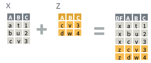
bind_rows(x, y)

where x and y:

are data frames
have the exact same column structure (names, order, & class)
you can add more than two data frames

Reshaping Data

Reshaping data includes:

turning rows into columns (aka pivot tables, cross tab query)
turning columns into rows

The go-to Tidyverse package for reshaping data frames is tidyr

Pivot Functions

pivot_longer()

pivot_wider()

More info and examples in the tidyr Pivoting Vignette

Group and Summarize

Step 1 (optional): group rows (i.e., change the unit of analysis)	group_by()
Step 2: Compute summaries for each group of rows	summarize() with: n(), mean(), median(), sum(), sd(), IQR(), first(), etc.

Example:

library(dplyr)
head(storms)

## # A tibble: 6 × 13
##   name   year month   day  hour   lat  long status       category  wind pressure
##   <chr> <dbl> <dbl> <int> <dbl> <dbl> <dbl> <fct>           <dbl> <int>    <int>
## 1 Amy    1975     6    27     0  27.5 -79   tropical de…       NA    25     1013
## 2 Amy    1975     6    27     6  28.5 -79   tropical de…       NA    25     1013
## 3 Amy    1975     6    27    12  29.5 -79   tropical de…       NA    25     1013
## 4 Amy    1975     6    27    18  30.5 -79   tropical de…       NA    25     1013
## 5 Amy    1975     6    28     0  31.5 -78.8 tropical de…       NA    25     1012
## 6 Amy    1975     6    28     6  32.4 -78.7 tropical de…       NA    25     1012
## # ℹ 2 more variables: tropicalstorm_force_diameter <int>,
## #   hurricane_force_diameter <int>

For each month, how many storm observations are saved in the data frame

storms |> 
  select(name, year, month, category) |>    ## select the columns we need
  group_by(month) |>                        ## group the rows by month
  summarize(num_storms = n())               ## for each group, report the count

## # A tibble: 10 × 2
##    month num_storms
##    <dbl>      <int>
##  1     1         70
##  2     4         66
##  3     5        201
##  4     6        779
##  5     7       1603
##  6     8       4440
##  7     9       7509
##  8    10       3077
##  9    11       1109
## 10    12        212

Intro to R Part 3:

Data Wrangling

Today’s Outline

Review from Part II

Plotting

Packages

Functions

Piping Syntax

Data Frames

Importing Data

Don’t Forget Cheatsheets!

Data Wrangling: What do we mean?

What is “tidy data”?

Are these data ‘tidy’?

Better Ways to Import Data

Data Wrangling with `dplyr`

Popular `dplyr` Functions

Row and Column Manipulations

Chaining dplyr functions

Example

Duplicate Function Names

R Notebooks

Notebook Exercise: Wrangle the Penguins

Data

Break!

Pro Tips

Renaming columns

Advanced `select()`

Joining and Merging Tables

Join tables on a common column

Joining Tables When the Column Name is Different

Stacking or Merging Data Frames

Reshaping Data

Pivot Functions

Group and Summarize

Notebook Exercise #2

END!

Intro to R Part 3:

Data Wrangling

Today’s Outline

Review from Part II

Plotting

Packages

Functions

Piping Syntax

Data Frames

Importing Data

Don’t Forget Cheatsheets!

Data Wrangling: What do we mean?

What is “tidy data”?

Are these data ‘tidy’?

Better Ways to Import Data

Data Wrangling with dplyr

Popular dplyr Functions

Row and Column Manipulations

Chaining dplyr functions

Example

Duplicate Function Names

R Notebooks

Notebook Exercise: Wrangle the Penguins

Data

Break!

Pro Tips

Renaming columns

Advanced select()

Joining and Merging Tables

Join tables on a common column

Joining Tables When the Column Name is Different

Stacking or Merging Data Frames

Reshaping Data

Pivot Functions

Group and Summarize

Notebook Exercise #2

END!

Data Wrangling with `dplyr`

Popular `dplyr` Functions

Advanced `select()`