Intro to R Part 4:

Data Wrangling 2 and ggplot

Andy Lyons
October 18, 2023

https://ucanr-igis.github.io/IntroR_Oct23/

Review

Data Wrangling

dropping columns
renaming columns
changing the order of columns
creating new columns with an expression
filtering rows
sorting rows
going from ‘long’ to ‘wide’ formats
joining data frames based on a common field
merging data frames together
splitting tables
aggregating rows into groups

Tidy data

Specialized packages for importing data

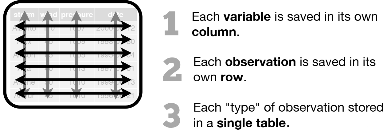
Row and column manipulations (`dplyr`)

subset rows	filter(), slice()
order rows	arrange()
pick column(s)	select(), pull()
add new columns	mutate()

Join and merge tables (`dplyr`)

join data frames on a column	left_join(), right_join(), inner_join()
stack data frames	bind_rows()

Reshape tables (`tidyr`)

convert rows to columns	pivot_wider()
turn columns into rows	pivot_longer()

Group rows and summarize (`dplyr`)

Step 1 (optional): group rows (i.e., change the unit of analysis)	group_by()
Step 2: Compute summaries for each group of rows	summarize() with: n(), mean(), median(), sum(), sd(), first(), etc.

Tips from Homework 3

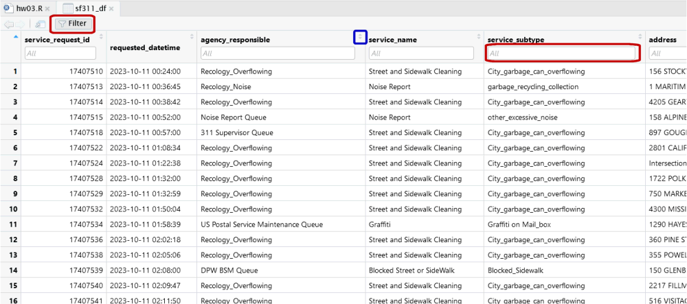
Exploring large data frames with the View pane:

Time Series Data

Challenges with date & time data

Often saved as formatted text:

October 5, 2023

5 Oct., 2023

10/05/2023

2023-10-05

Date formatting is often regional:

10-05-2023

05-10-2023

Date & Time Classes

Dates

Date class in R: Date

Current date:

x <- Sys.Date()
class(x)

## [1] "Date"

## [1] "2023-10-29"

Text to date:

as.Date("2023-09-25")

## [1] "2023-09-25"

Time

Date & time classes: POSIXct, POSIXlt

Sys.time()

## [1] "2023-10-17 19:28:42 PDT"

class(Sys.time())

## [1] "POSIXct" "POSIXt"

Supported Date Time Operations

format as text
extract date and time parts
Julian numbers
time zones automatically saved
intervals
date-time math
smart formatting on axes
etc.

Importing Date-Times

Convert Formatted Text to R Date/Time Object

Functions from lubridate:

ymd_hms(), ymd_hm(), ymd_h()

ydm_hms(), ydm_hm(), ydm_h()

mdy_hms(), mdy_hm(), mdy_h()

dmy_hms(), dmy_hm(), dmy_h()

Examples:

library(lubridate)
ymd_hms("2017-11-28T14:02:00")

## [1] "2017-11-28 14:02:00 UTC"

ymd_hms("2017-11-28T14:02:00", tz = "America/Los_Angeles")

## [1] "2017-11-28 14:02:00 PST"

Pro Tips:

To see the accepted time zone names, run OlsonNames()

Don’t name an object ‘date’

Combine Date/Time Parts

(x <- make_date(year = 2023, month = 10, day = 18))

## [1] "2023-10-18"

class(x)

## [1] "Date"

(y <- make_datetime (year = 2023, month = 10, day = 18, hour = 17, min = 15, sec = 0))

## [1] "2023-10-18 17:15:00 UTC"

class(y)

## [1] "POSIXct" "POSIXt"

Dealing with Missing Data

Step 1: Do I have missing values?

summary()

is.na(), !is.na()

Step 2: How do you want to handle missing data?

Option 1: Throw away the entire observation

tidyr::drop_na()

Option 2: Keep the observations but ignore missing values in column summaries

mean(x, na.rm = TRUE)

Option 3: Replace missing values with a constant

common replacement choices: 0, mean, median, etc.

mutate( new_col = if_else(…) )

tidyr::replace_na()

Option 4: Replace missing values with another column

mutate( new_col = if_else(…) )

mutate( new_col = coalesce(…) )

Option 5: Impute missing values from other rows

Sample methods:

repeat last value
linear interpolate
spline interpolate
etc.

See imputeTS or zoo packages.

Notebook Time: Clean CIMIS Weather Data

CIMIS Station #125, Arvin-Edison

Import data from CIMIS
Combine date part columns into a single date column
Reshape the data
Diagnose missing values
Replace missing values using the median and interpolation
Resample data

https://posit.cloud/content/6638058

After it opens:

Break!

Pro Tips

Chaing the Default Time Zone on Posit Cloud

The default time zone on Posit Cloud is UTC.

To mimic your local computer, you can change the default time zone:

Sys.setenv(TZ = "America/Los_Angeles")

Lags and Leads

To create a new column which includes lagged values, you can use

lag()
lead()

Saving Date-Times to Disk

Best Option: Use a file format that supports date and time classes

Examples:

native R files: (*.Rds, *.Rdata)
database files: sqlite, PostgreSQL
stats formats: Stata, SAS, SPSS

Second best: Use unambiguous character formatting

For file formats that don’t enforce data types (e.g., csv, txt, Excel), save dates as text formatted as:

yyyy-mm-dd

format(Sys.Date(), "%Y-%m-%d")

## [1] "2023-11-10"

Times can be formatted as ISO 8601. Example:

"2023-10-29T14:30:11-0700"

Note: the last five characters encode the time zone: -0700.

lubridate makes this easy with format_ISO8601()

lubridate::format_ISO8601(Sys.time(), usetz = TRUE)

## [1] "2023-11-10T10:09:01-0800"

ggplot

Example

Load Palmer Penguins data frame:

library(palmerpenguins)
head(penguins)

## # A tibble: 6 × 8
##   species island    bill_length_mm bill_depth_mm flipper_length_mm body_mass_g
##   <fct>   <fct>              <dbl>         <dbl>             <int>       <int>
## 1 Adelie  Torgersen           39.1          18.7               181        3750
## 2 Adelie  Torgersen           39.5          17.4               186        3800
## 3 Adelie  Torgersen           40.3          18                 195        3250
## 4 Adelie  Torgersen           NA            NA                  NA          NA
## 5 Adelie  Torgersen           36.7          19.3               193        3450
## 6 Adelie  Torgersen           39.3          20.6               190        3650
## # ℹ 2 more variables: sex <fct>, year <int>

Use ggplot to make a scatter plot:

ggplot(penguins, aes(x = flipper_length_mm, y = bill_length_mm, color = species)) +
  geom_point() +
  ggtitle("Bill Length vs Flipper Length for 3 Species of Penguins")

## Warning: Removed 2 rows containing missing values (`geom_point()`).

Anatomy of a ggplot

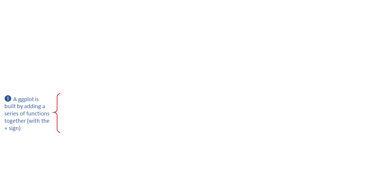
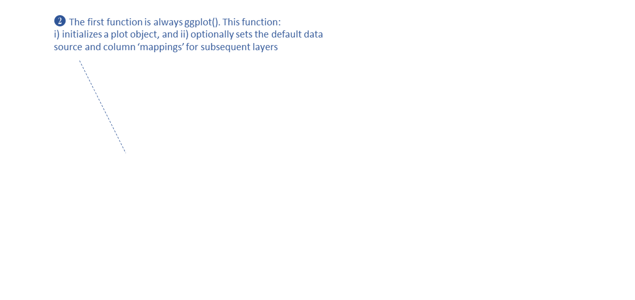
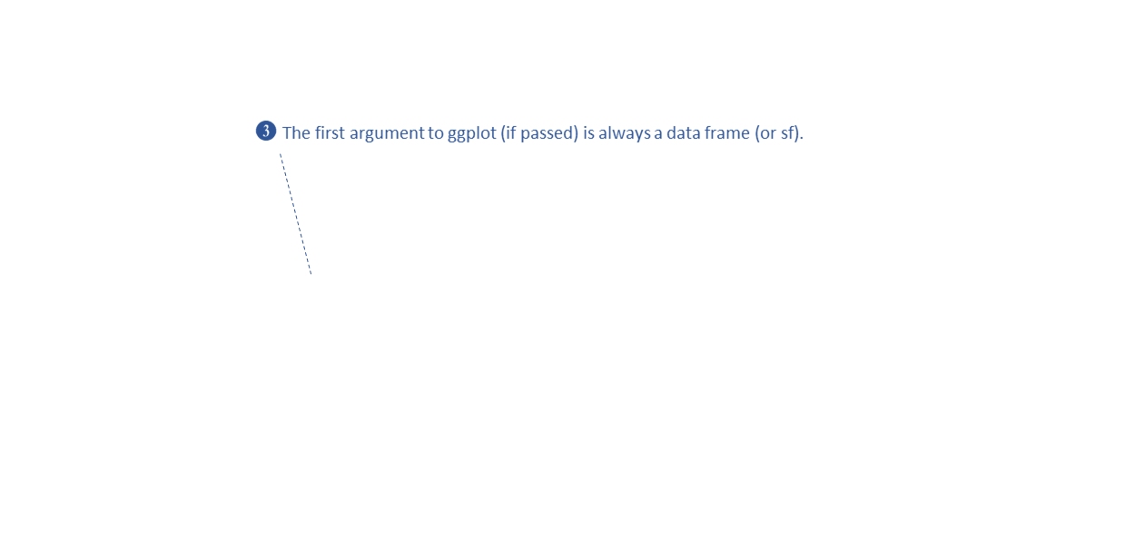
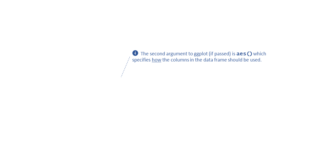
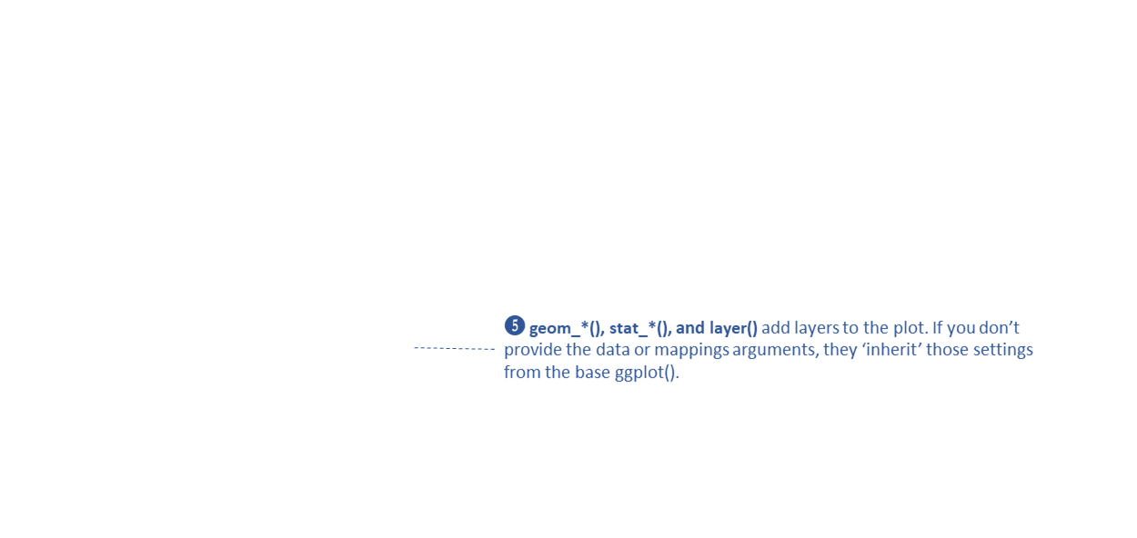
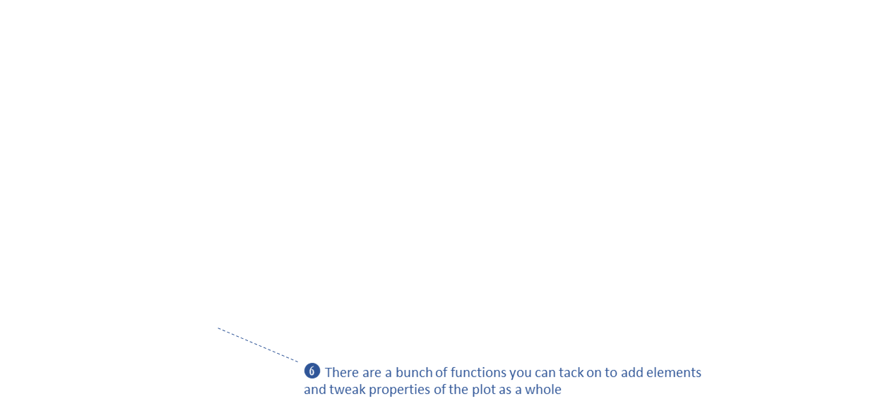
Maping Columns to Symbology Properties with `aes()`

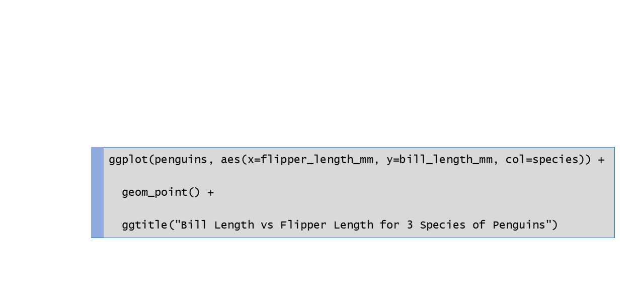
ggplot(penguins, aes(x = flipper_length_mm , y = bill_length_mm , color = species)) +
  geom_point() +
  ggtitle("Bill Length vs Flipper Length for 3 Species of Penguins")

aes() sets the default source for each visual property (or aesthetic) of the plot layers
- note you don’t need to put column names in quotes
some common visual properties:

x - where it falls along the x-axis
y - where it falls along the y-axis
color
fill
size

which visual properties are needed depends on the geom_xxxx() functions you use
only put in aes() the visual properties you want linked to the data

Geoms

geom_xxxx() functions add layers
drawn from the bottom up
some common geoms:

geom_point()

geom_bar()

geom_boxplot()

geom_histogram()

visual properties can be linked to a column in the data frame or manually specified

geom_point(col = pop_size)

geom_point(col = “red”)

visual properties are inherited (from aes())
each geom has default color palettes and legend settings

Example:

In the example below, note where geom_boxplot() gets its visual properties:

x and y are linked to columns in the dataframe and inherited from aes()
color, fill, and size are manually specified

ggplot(penguins, aes(x = species, y = bill_length_mm)) +
  geom_boxplot(color = "navy", fill = "yellow", size = 1.5)

## Warning: Removed 2 rows containing non-finite values (`stat_boxplot()`).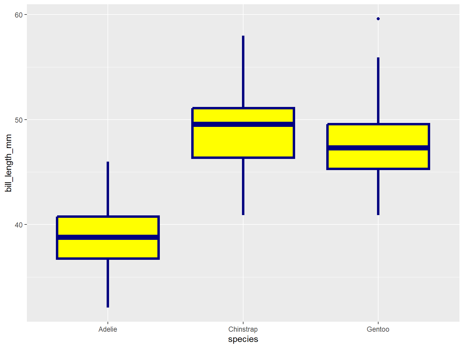

Adding visual elements to a plot

geom_xxxx() functions can also be used to add other graphic elements:

ggplot(penguins, aes(x = species, y = bill_length_mm)) +
  geom_boxplot(color = "navy", fill = "yellow", size = 1.5) +
  geom_hline(yintercept = 43.9, size=3, color="red") +
  geom_label(x = 3, y = 58, label = "Gentoo penguins \n are just the best!")

## Warning: Using `size` aesthetic for lines was deprecated in ggplot2 3.4.0.
## ℹ Please use `linewidth` instead.
## This warning is displayed once every 8 hours.
## Call `lifecycle::last_lifecycle_warnings()` to see where this warning was
## generated.

## Warning: Removed 2 rows containing non-finite values (`stat_boxplot()`).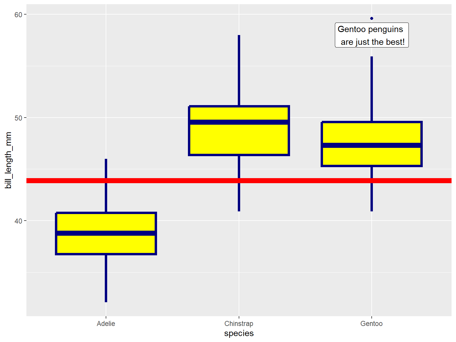

Notebook Time: Plotting the Palmer Penguins with ggplot

basic scatterplots
differentiating species by color
side-by-side plots with facets
box plots and histograms

End

Done!