R as a Fancy Calculator

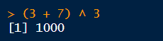
When you type an expression at the console and hit enter, R will evaluate the expression and print the result at the console.
When you save or assign the result of an expression to an object, R will not print the value at the console.
R has two assignment operators:

=
<-
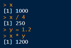
To view the value of an object, you can enter it at the console.

Once defined, an object can be used in subsequent expressions.

Objects are stored in memory. They will disappear when you shut down R (unless you tell RStudio to auto-save and reload objects in memory).
Every object has a data type or class.

Common data types:

numeric
character
factor
date
data frame, tibble
matrix
list

Naming Objects

The rules for naming objects are pretty flexible. You can use numbers, letters, and most special characters.

A few rules to take note of:

Can’t start with a number: 3pieces
Hyphens and spaces not allowed: first name, last-name
Don’t use the name of a built-in function, constant, or keyword: c, pi

Naming Styles

There are a handful of popular naming styles. Pick one that you like, and be consistent!

Style	Example
alllowercase	adjustcolor
period.separated	shoe.size
underscore_separated (aka snake case)	numeric_version
lowerCamelCase	addTaskCallback
UpperCamelCase	SignatureMethod

Scripts

Top five advantages of using scripts over the console:

Easier to write (and fix!) your code
You can add comments to remind yourself what each command is doing
Reuse your own code
You can add loops and if-then statements later on
Tell your friends you’re a coder!

Notebooks

Similar to scripts, but can also include paragraph text, headings, pictures, formatting, etc.

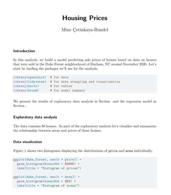
R supports RMarkdown and Quarto markdown (similar).

R code is included in “code chunks” that get executed whenever you render the Notebook.

Notebooks are great when the desired output is an HTML document, PDF, Word Doc, etc.

For code that you want to repeat often, use a script.

Functions

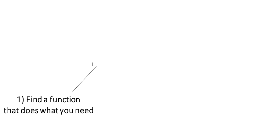
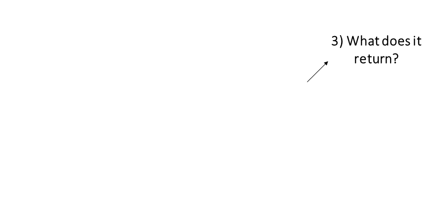
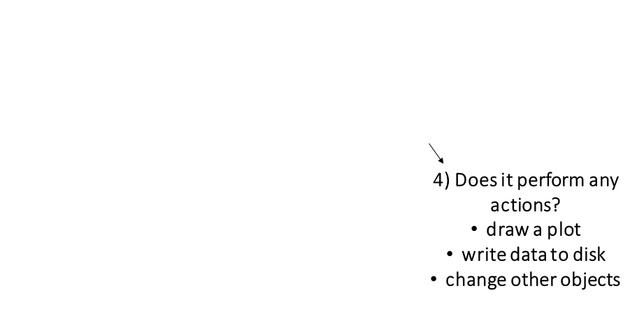
The keys to R’s superpowers are functions! There are four things you need to know to use a function:

What Do Functions Return?

numbers
dates
text
data frames and matrices
spatial data
plots
trained regression models
HTML widgets
another function that returns a color ramp
a drone image collection metadata record
⇒ almost anything you can think of can be returned by a function!!
⇒ anything returned by a function can also be saved to an object

Which function should I use?

Finding the right R function, half the battle is.

- Jedi MasteR Yoda

Ask your friends

Ask Google / ChatGPT

Cheatsheets!

Function Help

Every function has a help page. To get to it enter ? followed by the name of the function (without parentheses):

?rnorm

Function Arguments

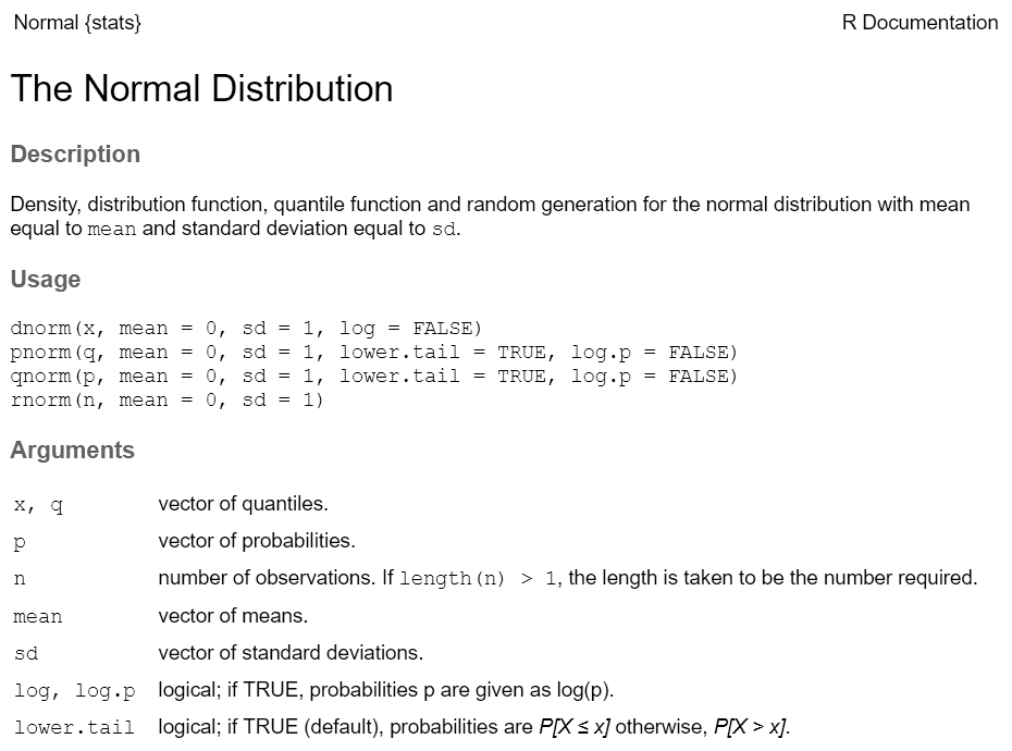
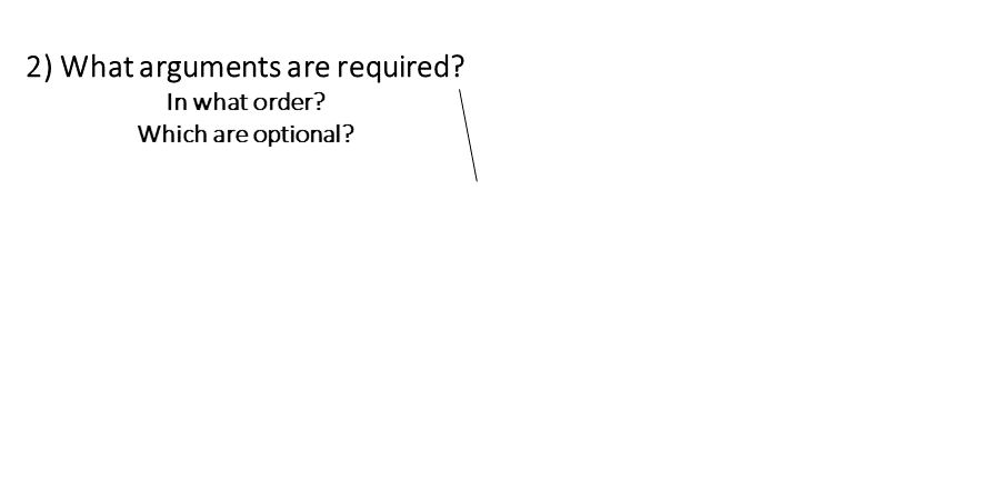
Most functions take arguments. Arguments can be required or optional (i.e. have a default value).

See the function’s help page to determine which arguments are expected. Example:

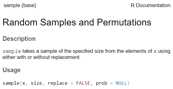
x and size have no default value → they are required

replace and prob have default values → they are optional

To name or not to name your arguments? That is the question.

All arguments have names. You can explicitly name arguments when calling a function as follows:

rnorm(n = 100, mean = 10, sd = 0.3)

Benefits of naming your arguments:

Helps you remember what each argument is
You can enter then in any order
You can skip arguments if you’re happy with the default value

But you can omit argument names if you pass them in the order expected and don’t skip any.

rnorm(500, 50, 3)  ## generate 500 normally distributed random
                   ## numbers with a mean of 50 and stand dev = 3.

R Packages

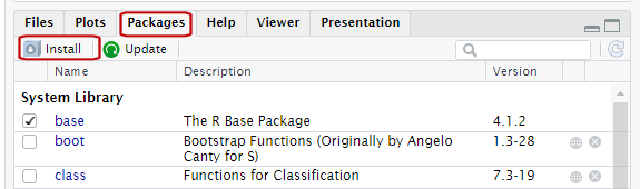
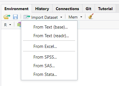
Packages are what R calls extensions or add-ons.

What’s in a package?

additional functions!
function help pages
tutorials (Vignettes)
datasets

Where do you find them?

people in your field
CRAN - Task Views
CRAN - List of all packages by name
publications
blog posts (e.g., R packages for Agricultural Research)

Installing and Using Packages

Three simple steps to use the functions in a package:

Figure out which package you need
Install (i.e., download) it (just once)

Load it into memory (must do this every time you start RStudio)

library(dplyr)

Piping

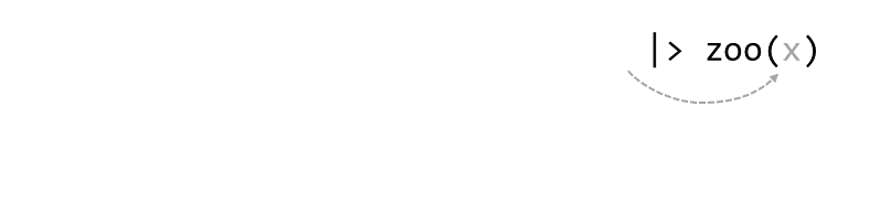
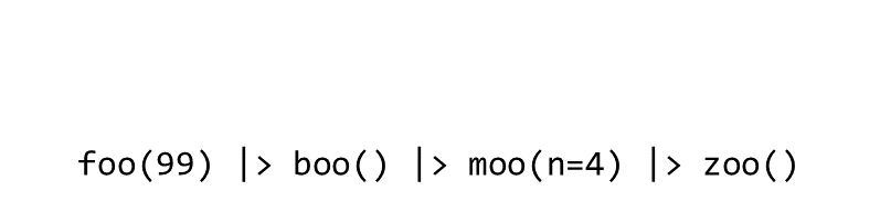
Piping syntax is an alternative syntax for chaining together functions.

With piping, you use the pipe operator |> (or %>%) to ‘feed’ the result of one function into the next function.

Piping allows the results of one function to be passed as the first argument of the next function. Hence a series of commands to be written like a sentence.

This generally requires functions that have been written to make changes to whatever object was passed in first argument, and return it.

Example

Consider the expression:

zoo(moo(boo(foo(99)),n=4))

Piping Tips and Tricks

Keyboard shortcut for inserting the pipe operator: ctrl + shift + m

You can tell RStudio which pipe to insert under Global Options >> Code

|> (‘native’ pipe introduced R4.0)

%>% (from magrittr package)

To split a chain of functions across multiple lines, end each line with a pipe operator:

seq(1, 10, 0.1) |> 
  log() |> 
  sum()

## [1] 141.4023

If the receiving function requires additional arguments, just add them starting with the 2nd argument (or use named arguments):

runif(5) |> round(2)

## [1] 0.41 0.97 0.08 0.07 0.26

Same Function Name, Different Packages

Occasionally two or more packages will have different functions that use the same name.

When this happens, R will use whichever one was loaded first.

Best practice: use the package name and the :: reference to specify which package a function is from.

x <- sp::over()
x <- grDevices::over()

y <- raster::select()
y <- dplyr::select()

When you use the package_name::function_name syntax, you don’t actually have to first load the package with library().

Resolving Name Conflicts with the conflicted Package

When you call a function that exists in multiple packages, R uses whichever package was loaded first.

The conflicted package helps you avoid problems with duplicate function names, by specifying which one to prioritize no matter what order they were loaded.

library(conflicted)

# Set conflict preference
conflict_prefer("filter", "dplyr")
conflict_prefer("count", "dplyr")
conflict_prefer("select", "dplyr")

# From here on out, anytime we call select() or filter(), R will
# always use the dplyr version.

Vectors

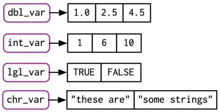
Vectors are R objects that contain multiple elements of the same class.

Example:

i = 4:12
i

## [1]  4  5  6  7  8  9 10 11 12

More examples:

Making Vectors

In general, you need to use a function or operator to create a vector.

Example 1: Create a sequence of numbers with the : operator:

1:10

##  [1]  1  2  3  4  5  6  7  8  9 10

Example 2: rep() function

rep("Quercus", 5)

## [1] "Quercus" "Quercus" "Quercus" "Quercus" "Quercus"

Example 3: Random number functions

## Generate normally distributed random numbers
rnorm(5)

## [1] -1.6891683 -1.1048986 -0.6000753  2.2828762  0.1296368

## R has a built-in constant with the names of the months
month.name

##  [1] "January"   "February"  "March"     "April"     "May"       "June"     
##  [7] "July"      "August"    "September" "October"   "November"  "December"

## Sample three months at random
sample(month.name, 3)

## [1] "November" "December" "January"

Example 4: Manually combine elements with c()

yn <- c(TRUE, FALSE, TRUE)
yn

## [1]  TRUE FALSE  TRUE

How big is my vector?

length(yn)

## [1] 3

“Vectorized” Functions: The Best Thing Since Sliced Bread

Many R functions and math operators are vectorized (i.e., operate on each individual element).

Example

First we create two numeric vectors:

x = 0:4
y = 11:15

Are sin() & cos() vectorized?

sin(x)

## [1]  0.0000000  0.8414710  0.9092974  0.1411200 -0.7568025

cos(y)

## [1]  0.004425698  0.843853959  0.907446781  0.136737218 -0.759687913

Addition (and all math functions) is vectorized:

x + 1

## [1] 1 2 3 4 5

x + y

## [1] 11 13 15 17 19

Aggregate functions

Functions that accept a vector and spit out a single value are called aggregate functions.

## Sum
sum(x)

## [1] 10

## Mean
mean(x)

## [1] 2

## Standard deviation
sd(x)

## [1] 1.581139

Subset Vectors

To extract a single element from a vector, you can use square bracket notation. Inside the square brackets, enter an expression that specifies which elements to return.

my_vector[ expression-which-identifies-specific-elements
]

Option 1. Subset with indices

state.abb[5]

## [1] "CA"

To return multiple elements, pass a vector of indices.

state.abb[5:7]

## [1] "CA" "CO" "CT"

state.abb[c(10, 4, 6, 9)]

## [1] "GA" "AR" "CO" "FL"

Option 2: Subset with logicals

You can also insert a vector of logical values (TRUE/FALSE) in the brackets. R will return the corresponding element for the TRUE values.

month.name[c(FALSE, FALSE, TRUE, FALSE, FALSE, FALSE, FALSE, FALSE, FALSE, FALSE, FALSE, FALSE)]

## [1] "March"

Better still, use an expression that returns a vector of logical values:

Example: Pull all out the months that start with ‘M’.

## View the first letter of each month
substr(month.name, 1, 1)

##  [1] "J" "F" "M" "A" "M" "J" "J" "A" "S" "O" "N" "D"

## Use that to find all the months that start with 'M'
month.name[substr(month.name, 1, 1) == "M"]

## [1] "March" "May"

Tabular Data

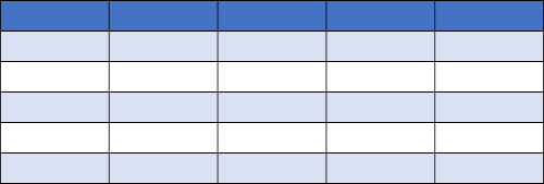
R has two data classes that organize data in rows and columns:

data frames
matrices

Rows and Columns by any other name….

rows

aka:
- record
- case
- observation
- feature (spatial)

columns

aka: variable, field

##   Sepal.Length Sepal.Width Petal.Length Petal.Width Species
## 1          5.1         3.5          1.4         0.2  setosa
## 2          4.9         3.0          1.4         0.2  setosa
## 3          4.7         3.2          1.3         0.2  setosa
## 4          4.6         3.1          1.5         0.2  setosa
## 5          5.0         3.6          1.4         0.2  setosa
## 6          5.4         3.9          1.7         0.4  setosa

Key concepts

columns of a data frame are vectors
columns have names
you can refer to columns by their name or position
data frames and tibbles are essentially equivalent

Pulling out a Single Column

To get an individual column, use $

head(trees)

##   Girth Height Volume
## 1   8.3     70   10.3
## 2   8.6     65   10.3
## 3   8.8     63   10.2
## 4  10.5     72   16.4
## 5  10.7     81   18.8
## 6  10.8     83   19.7

trees$Height

##  [1] 70 65 63 72 81 83 66 75 80 75 79 76 76 69 75 74 85 86 71 64 78 80 74 72 77
## [26] 81 82 80 80 80 87

trees$Height |> summary()

##    Min. 1st Qu.  Median    Mean 3rd Qu.    Max. 
##      63      72      76      76      80      87

Subsetting rows and columns

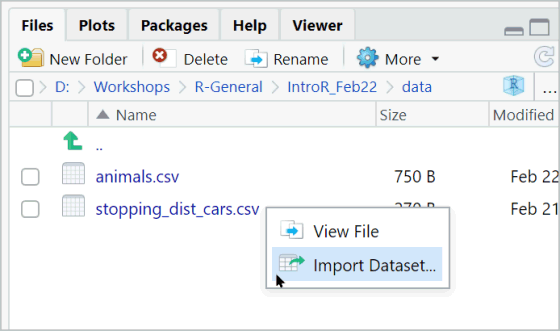
You can use square bracket notation or tidyverse methods (dplyr).

trees[10:12, c("Girth", "Volume")]

##    Girth Volume
## 10  11.2   19.9
## 11  11.3   24.2
## 12  11.4   21.0

Fundamentals of Coding with R

Outline

R as a Fancy Calculator

Naming Objects

Naming Styles

Scripts

Notebooks

Functions

What Do Functions Return?

Which function should I use?

Function Help

Function Arguments

To name or not to name your arguments? That is the question.

R Packages

What’s in a package?

Where do you find them?

Installing and Using Packages

Piping

Example

Piping Tips and Tricks

Same Function Name, Different Packages

Vectors

Making Vectors

“Vectorized” Functions: The Best Thing Since Sliced Bread

Aggregate functions

Subset Vectors

Option 1. Subset with indices

Option 2: Subset with logicals

Tabular Data

Rows and Columns by any other name….

Key concepts

Pulling out a Single Column

Subsetting rows and columns

Importing Data: RStudio’s Import Dataset Wizard

End!