Exercise 1: Import & Plot Vector Data

Spatial Data Fundamentals in R

Summary

In this exercise we will import some layers for Yosemite National Park from local and online sources, do some cleaning and filtering, and plot them.

Setup

library(sf)
library(here)
library(dplyr)
library(arcgislayers)

View Available Layers for Yosemite National Park

First let’s look at layers in the ./exercises/data folder, by passing the directory to sf::st_layers(). This will show us the Shapefiles but not layers that are in ‘containers’, like file geodatabases, geojson files, etc.

## View spatial layers in the data folder.
st_layers(here("./exercises/data"))

Import a Shapefile

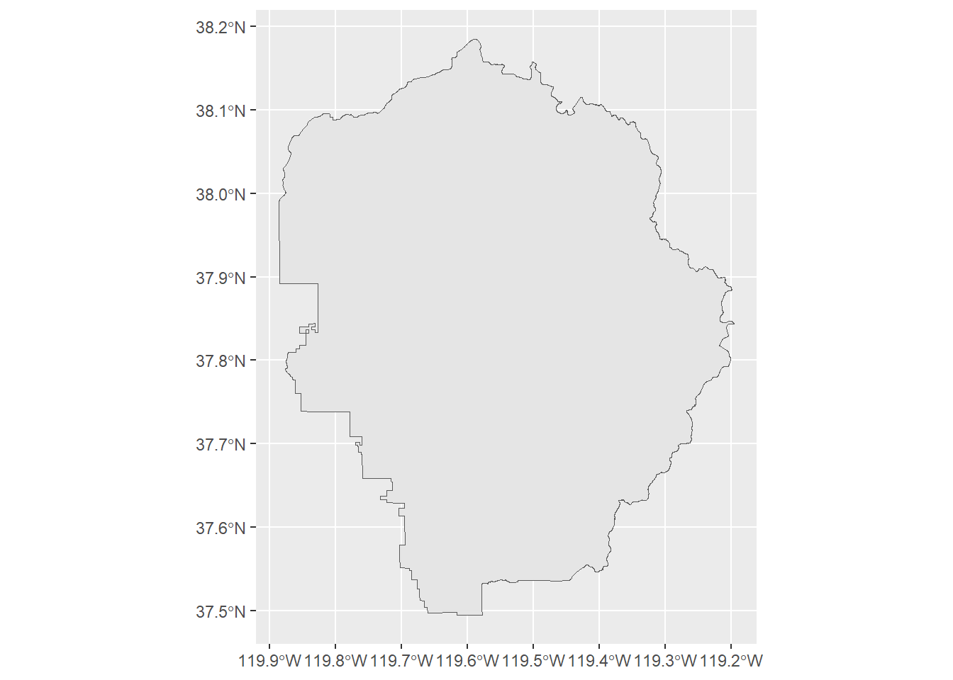
Import the ‘yose_boundary’ layer (a Shapefile).

Note: if we use the layer argument we don’t need to include the .shp extension.

yose_bnd_ll <- st_read(dsn = here("./exercises/data"), 
                       layer = "yose_boundary")

Reading layer `yose_boundary' from data source 
  `D:\Workshops\R-Spatial2\SpatialDataFundamentals_2hr\SpatialDataR\exercises\data' 
  using driver `ESRI Shapefile'
Simple feature collection with 1 feature and 11 fields
Geometry type: POLYGON
Dimension:     XY
Bounding box:  xmin: -119.8864 ymin: 37.4947 xmax: -119.1964 ymax: 38.18515
Geodetic CRS:  North_American_Datum_1983

Naming Objects

The naming convention throughout this exercise is to name objects using a sequence of tags separated by ’_’.

For example, yose_bnd_ll consists of:

yose - all Yosemite layers start with this
bnd - tell me this the park boundary
ll - lat-long coordinates

View the class of yose_bnd_ll:

## View the class of the object we just created
class(yose_bnd_ll)

[1] "sf"         "data.frame"

We see that yose_bnd_ll is both a sf object (simple feature data frame) as well as a data.frame. This means we should be able to use the functions designed for either of those objects.

Next, view the properties of yose_bnd_ll by simply running it by itself:

yose_bnd_ll

Simple feature collection with 1 feature and 11 fields
Geometry type: POLYGON
Dimension:     XY
Bounding box:  xmin: -119.8864 ymin: 37.4947 xmax: -119.1964 ymax: 38.18515
Geodetic CRS:  North_American_Datum_1983
  UNIT_CODE
1      YOSE
                                                                            GIS_NOTES
1 Lands - http://landsnet.nps.gov/tractsnet/documents/YOSE/METADATA/yose_metadata.xml
               UNIT_NAME  DATE_EDIT STATE REGION GNIS_ID     UNIT_TYPE
1 Yosemite National Park 2016-01-27    CA     PW  255923 National Park
  CREATED_BY                                               METADATA PARKNAME
1      Lands http://nrdata.nps.gov/programs/Lands/YOSE_METADATA.xml Yosemite
                        geometry
1 POLYGON ((-119.8456 37.8327...

Plot the Yosemite Boundary

library(ggplot2)
ggplot() +
  geom_sf(data = yose_bnd_ll)

CHALLENGE

Import the Historic Points Shapefile and plot it.

yose_hp_ll <- st_read(dsn = here("./exercises/data"), 
                       layer = "yose_historic_pts")

Reading layer `yose_historic_pts' from data source 
  `D:\Workshops\R-Spatial2\SpatialDataFundamentals_2hr\SpatialDataR\exercises\data' 
  using driver `ESRI Shapefile'
Simple feature collection with 35 features and 1 field
Geometry type: POINT
Dimension:     XY
Bounding box:  xmin: -119.8447 ymin: 37.51356 xmax: -119.2165 ymax: 38.08368
Geodetic CRS:  WGS 84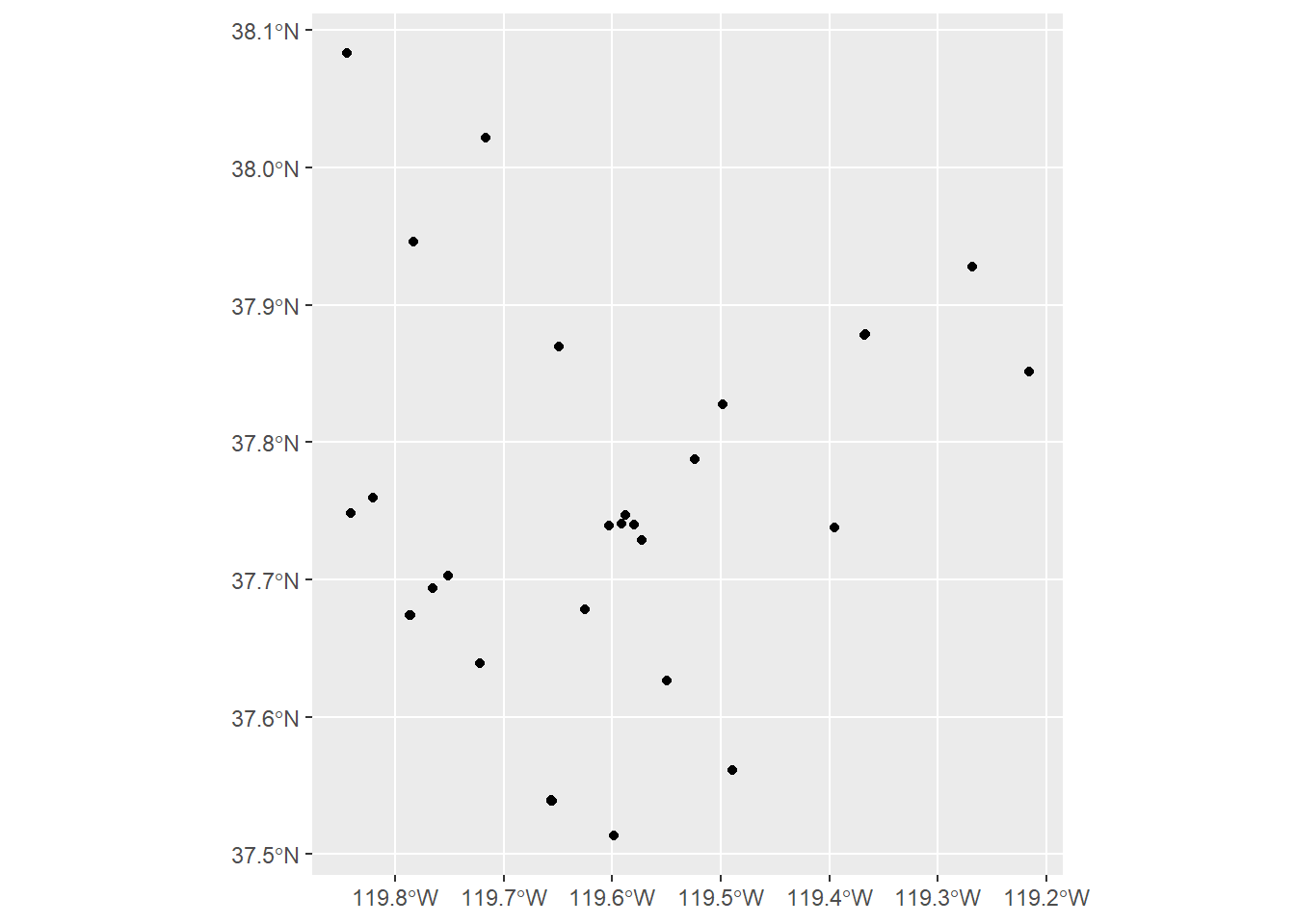

ggplot() +  geom_sf(data = yose_hp_ll)

Import the Yosemite Points-of-Interest (POI)

Next, import the points-of-interest Shapefile, and overlay it on top of the park boundary.

## Import the yose_poi.shp
yose_poi_ll <- st_read(dsn="./data", layer="yose_poi")

Reading layer `yose_poi' from data source 
  `D:\Workshops\R-Spatial2\SpatialDataFundamentals_2hr\SpatialDataR\exercises\data' 
  using driver `ESRI Shapefile'
Simple feature collection with 2720 features and 30 fields
Geometry type: POINT
Dimension:     XY
Bounding box:  xmin: 246416.2 ymin: 4153717 xmax: 301510.7 ymax: 4208419
Projected CRS: NAD83 / UTM zone 11N

head(yose_poi_ll)

ggplot() + 
  geom_sf(data = yose_poi_ll) +
  geom_sf(data = yose_bnd_ll, fill = NA, color = "darkgreen", size = 1) +
  labs(title = "Yosemite National Park Points of Interest")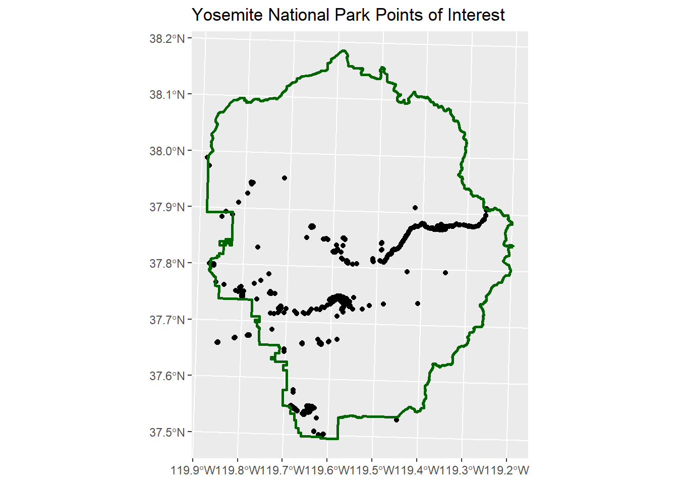

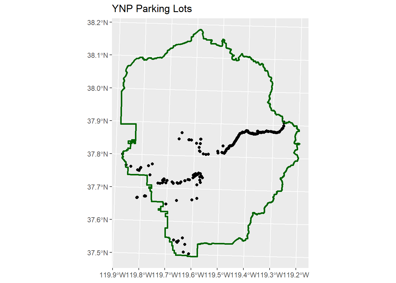
Subset the Points of Interest

Because sf objects are just data frames, we can use standard data frame functions to explore and manipulate them.

For example to tabulate the unique values in the POITYPE column:

table(yose_poi_ll$POITYPE)


    Backcountry Campsite               Campground         Campground Kiosk 
                       9                       15                       10 
                Campsite                   Church         Entrance Station 
                    1219                        1                        9 
            Food Service              Gas Station                 Hospital 
                      11                        4                        1 
                 Lodging                   Market                   Museum 
                     789                        5                        3 
                   Other              Parking Lot              Picnic Area 
                      41                      259                       18 
             Post Office Private Residence Rental          Public Restroom 
                       3                      122                       31 
                Restroom                   Stable                    Store 
                      97                        1                        2 
               Trailhead           Visitor Center 
                      65                        5

We can use this field to plot just the parking lots:

yose_parking_lots_ll <- yose_poi_ll |> 
  filter(POITYPE == "Parking Lot")

dim(yose_parking_lots_ll)

[1] 259  31

ggplot() + 
  geom_sf(data = yose_parking_lots_ll) +
  geom_sf(data = yose_bnd_ll, fill = NA, color = "darkgreen", size = 1) +
  labs(title = "YNP Parking Lots")

Import Roads from a Geodatabase

You can import layers from an ESRI file geodatabase using the sf package. In this case, the source is the folder containing the geodatabase.

Import the Yosemite’s roads from a geodatabase. First find the gdb directory:

gdb_fn <- here::here("./exercises/data/yose_roads.gdb")
file.exists(gdb_fn)

[1] TRUE

View the layers in this source:

st_layers(gdb_fn)

Driver: OpenFileGDB 
Available layers:
      layer_name     geometry_type features fields             crs_name
1 Yosemite_Roads Multi Line String      823     40 NAD83 / UTM zone 11N

Import the Yosemite_Roads layer:

## Import the 'Yosemite_Roads' layer  (case sensitive!)
yose_roads_utm11n <- st_read(gdb_fn, layer="Yosemite_Roads")

Reading layer `Yosemite_Roads' from data source 
  `D:\Workshops\R-Spatial2\SpatialDataFundamentals_2hr\SpatialDataR\exercises\data\yose_roads.gdb' 
  using driver `OpenFileGDB'
Simple feature collection with 823 features and 40 fields
Geometry type: MULTILINESTRING
Dimension:     XY
Bounding box:  xmin: 234658.1 ymin: 4139484 xmax: 324852.6 ymax: 4250252
Projected CRS: NAD83 / UTM zone 11N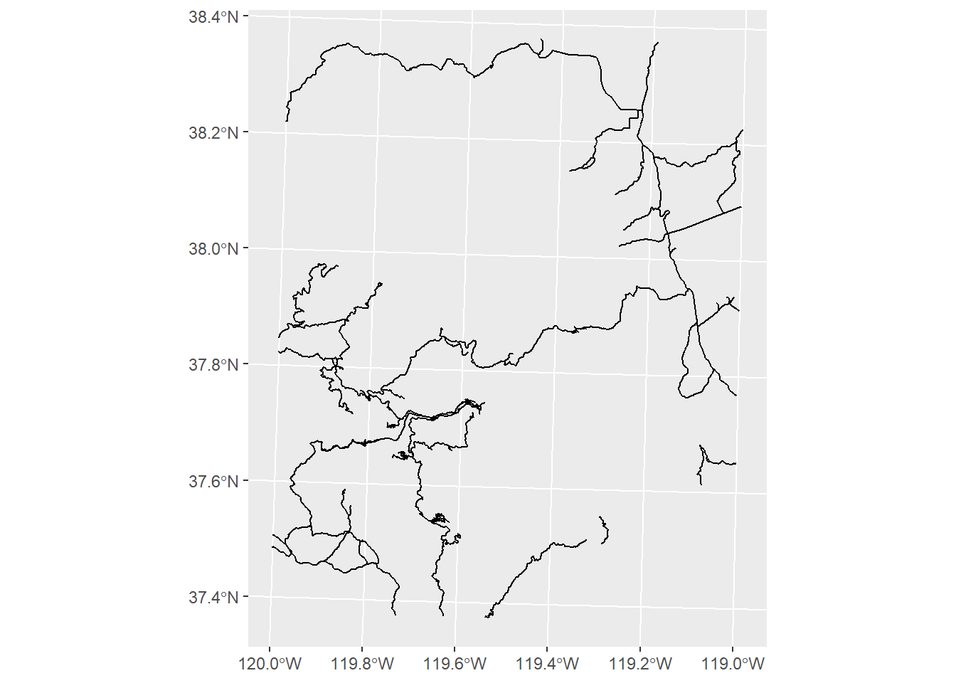

ggplot() + geom_sf(data = yose_roads_utm11n)

Customizing the axes and graticules

As can be seen above, geom_sf() will display geographic coordinates on the axes, even if the data are projected.

To change the CRS for the coordinates on the axes, add coord_sf() and pass a CRS object for the datum argument.

ggplot() + 
  geom_sf(data = yose_roads_utm11n) + 
  coord_sf(datum = st_crs(yose_roads_utm11n))

CHALLENGE

Plot just the primary roads.

yose_roads_pri_utm11n <- yose_roads_utm11n |> 
  filter(RDCLASS == "Primary")

dim(yose_roads_pri_utm11n)

[1] 180  41

ggplot() + 
  geom_sf(data = yose_roads_pri_utm11n, color = "darkgray") +
  geom_sf(data = yose_bnd_ll, fill = NA, color = "darkgreen", size = 1) +
  labs(title = "YNP Primary Roads")

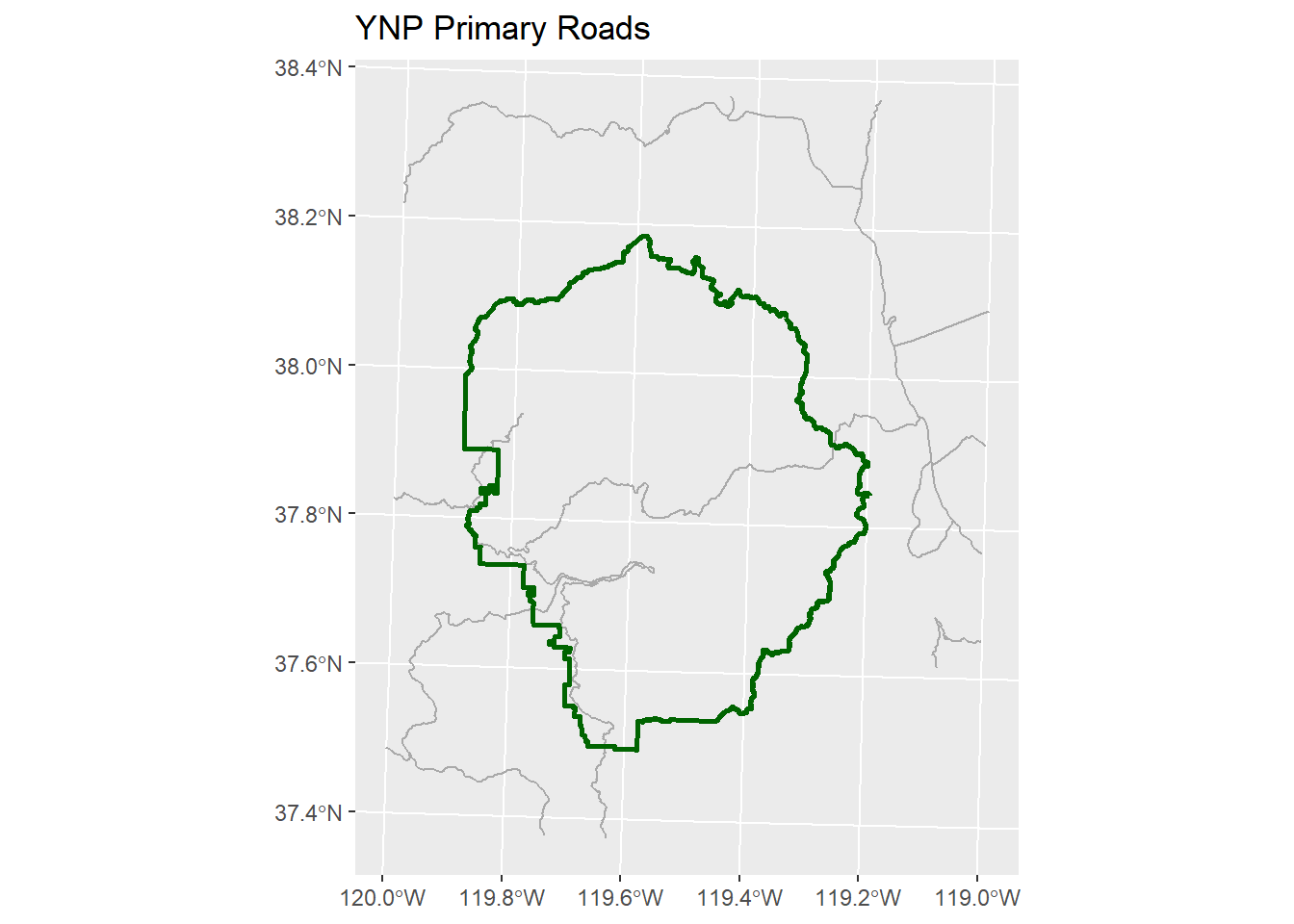
Extract the roads that fall within the park

To plot just the roads in the park, we can do an intersection.

Note however intersections require the layers to be in the same CRS. Here we can project the park boundary to match the roads.

yose_bnd_utm11n <- yose_bnd_ll |> 
  st_transform(st_crs(yose_roads_utm11n))

yose_roads_park_utm11n <- yose_roads_utm11n |> 
  st_intersection(yose_bnd_utm11n)

Warning: attribute variables are assumed to be spatially constant throughout
all geometries

dim(yose_roads_utm11n)

[1] 823  41

dim(yose_roads_park_utm11n)

[1] 638  52

ggplot() + 
  geom_sf(data = yose_roads_park_utm11n, color = "darkgray") +
  geom_sf(data = yose_bnd_ll, fill = NA, color = "darkgreen", size = 1) +
  labs(title = "YNP Park Roads")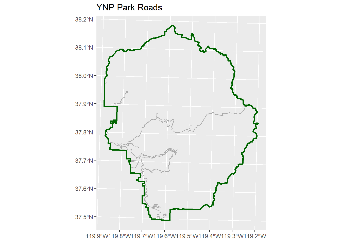

Import Watersheds from ArcGIS Online

Let’s import the watersheds. These are available from the California State Water Resources Control Board (SWRCB) which shares the Feature Service through their ArcGIS Enterprise portal:

https://gispublic.waterboards.ca.gov/portal/home/item.html?id=816893ddab33434989eda92dbc0e126f

Step 1 is to find the URL for the FeatureServer (on the website).

Then we can import it using arcgislayers.

library(arcgislayers)

## URL for a publicly available Feature Server
pws_featsrv_url <- "https://gispublic.waterboards.ca.gov/portalserver/rest/services/Hosted/CalWater/FeatureServer"

## Create a FeatureServer object
pws_featsrv_fs <- arc_open(pws_featsrv_url)
pws_featsrv_fs

<FeatureServer <6 layers, 0 tables>>
CRS: 3857
Capabilities: Query,Sync,Extract
  0: CalWater_Hydrologic_Region (esriGeometryPolygon)
  1: CalWater_Hydrologic_Unit (esriGeometryPolygon)
  2: CalWater_Hydrologic_Subarea (esriGeometryPolygon)
  3: CalWater_Hydrologic_Area (esriGeometryPolygon)
  4: CalWater_Hydrologic_SPW (esriGeometryPolygon)
  5: CalWater_Hydrologic_PW (esriGeometryPolygon)

## List the layers available
arcgislayers::list_items(pws_featsrv_fs)

## Create a FeatureLayer object
pws_featsrv_fl <- arcgislayers::get_layer(pws_featsrv_fs, id = 5)
pws_featsrv_fl

<FeatureLayer>
Name: CalWater_Hydrologic_PW
Geometry Type: esriGeometryPolygon
CRS: 3857
Capabilities: Query,Sync,Extract

## If you want you can view the fields
# list_fields(pws_featsrv_fl)

## Download the polygons and plot
## THIS MAY OVERWHELM POSIT CLOUD SO HAS BEEN COMMENTED OUT. 
# pws_ca_sf <- arc_select(pws_featsrv_fl) 
# dim(pws_ca_sf)
# ggplot() + geom_sf(data = pws_ca_sf)

## Alternative: display a saved version
knitr::include_graphics(here("./exercises/images/ca_planning_watersheds.png"))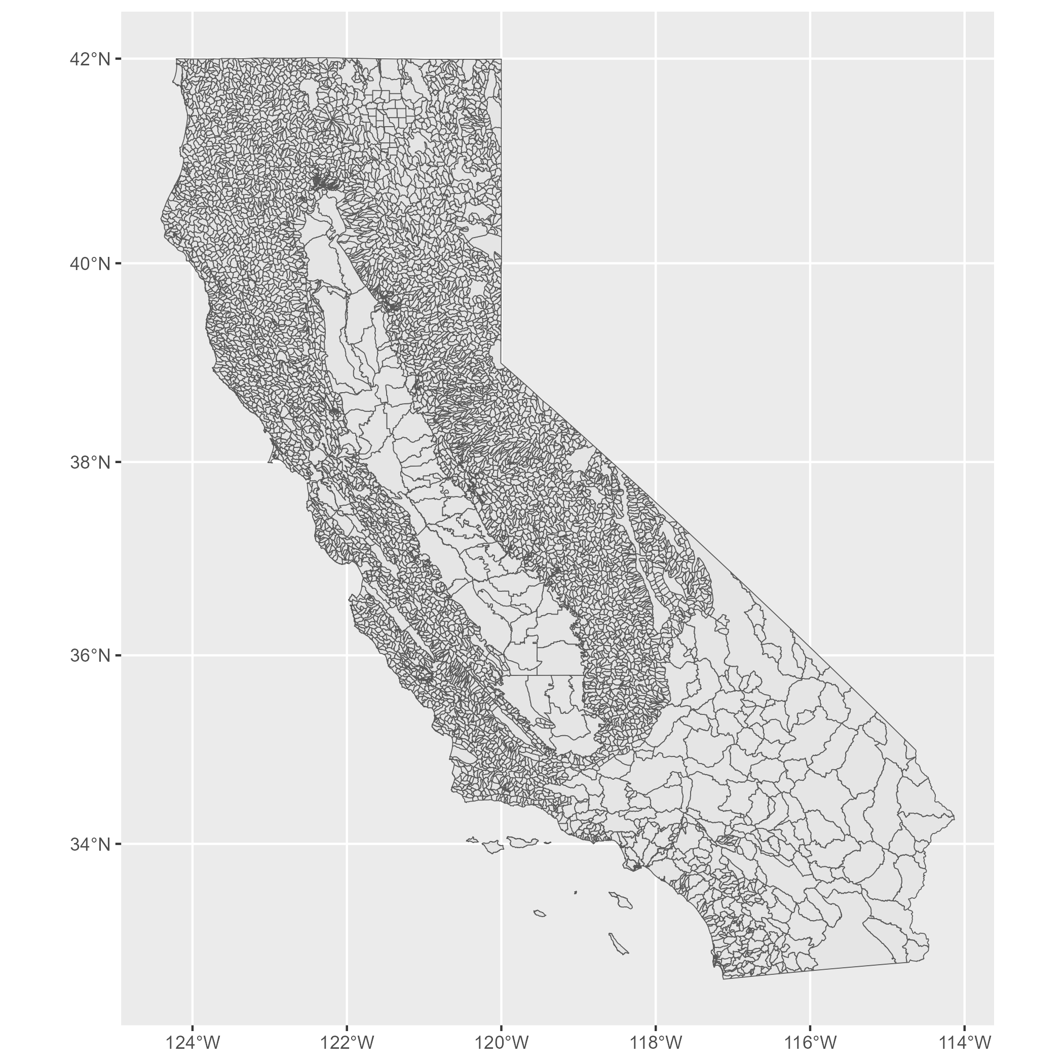

Import with a Spatial Filter

Fortunately for us, arc_select() supports two ways to filter the data on the server.

where: pass a ‘WHERE’ expression for an attribute filter
filter_geom: pass a bounding box for a spatial filter

Here we’ll apply a spatial filter to get only the planning watersheds for Yosemite.

pws_yose_sf <- arc_select(pws_featsrv_fl,
                          filter_geom = st_bbox(yose_bnd_ll))

Registered S3 method overwritten by 'jsonify':
  method     from    
  print.json jsonlite

nrow(pws_yose_sf)

[1] 175

ggplot() +
  geom_sf(data = pws_yose_sf) +
  geom_sf(data = yose_bnd_ll, size = 2, fill = NA, color = "navy")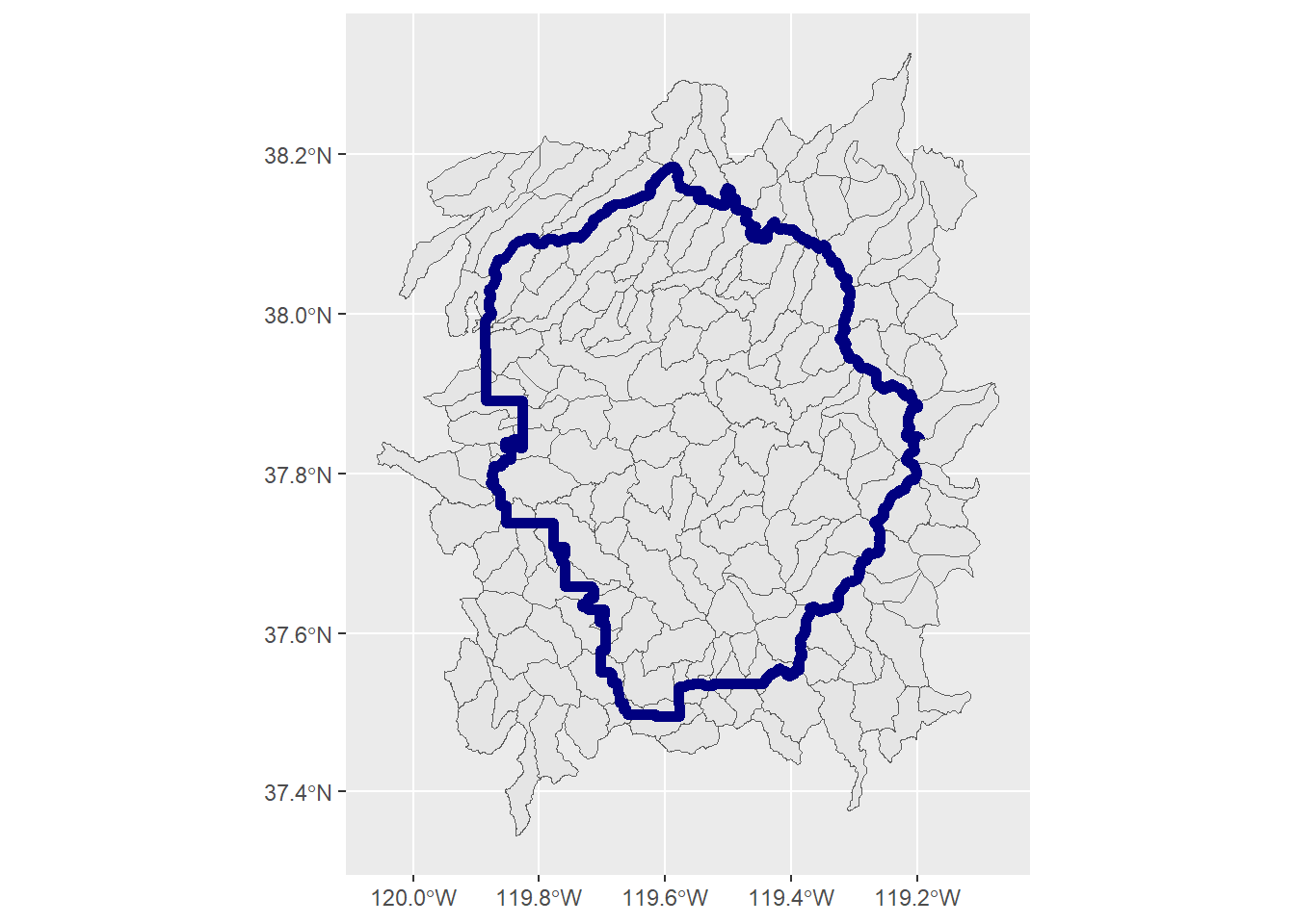

CHALLENGE

Import another layer and overlay it.

You can either select another layer from the ‘data’ folder, or import one from the YNP Minimum Essential Dataset (MED) feature layer (search & rescue):

Base Data - Yosemite National Park MED
https://www.arcgis.com/home/item.html?id=0c1bebf618d0425ba3181a5b0fcac821

## Your answer here