Working with Climate Data in R with caladaptR
Andy Lyons
May 2021

Andy Lyons
May 2021
Cal-Adapt is California’s official portal for peer-reviewed climate data.
Datasets are selected with guidance and priorities from California State agencies.
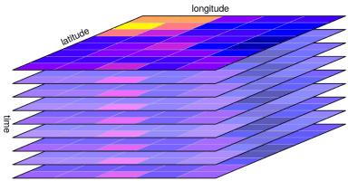
Projected Climate Data:
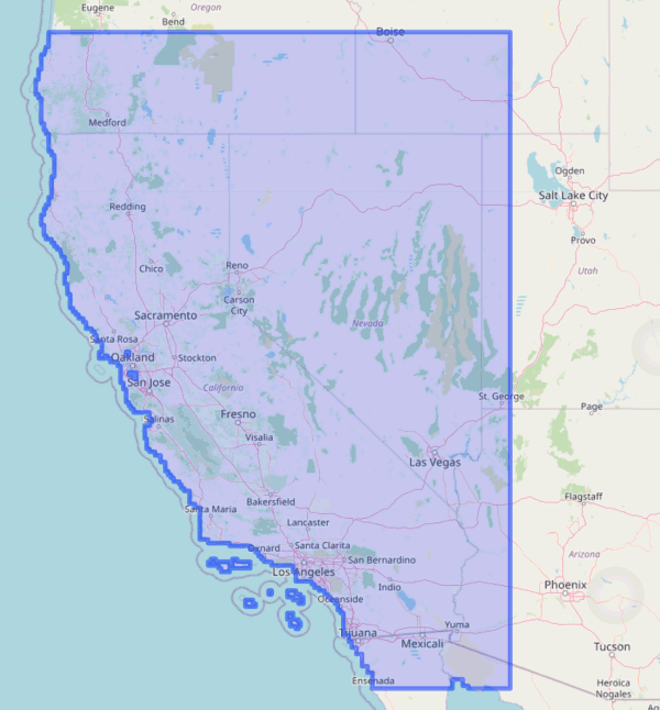
Extent of LOCA downscaled climate data layers:

![]()
![]()
![]()
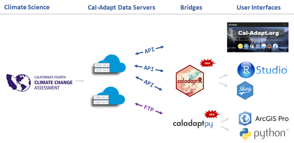
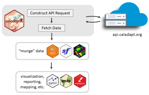
caladaptr is an API client package
The user is expected to know:
No problem!
cap1_db <- cap1 %>%
ca_getvals_db(db_fn = "c:/data/mydata.sqlite", db_tbl = "temp_min_max")No problem!
cap1_tifs <- cap1 %>%
ca_getrst_stars(out_dir = "c:/data/tifs")ca_read_stars()

See samples:
## Install caladaptr.apps and all dependent packages
remotes::install_github("ucanr-igis/caladaptr.apps")
library(caladaptr.apps)

## Launch the time series app
ca_launch("timeseries")

## Launch the projected chill portions app
ca_launch("chill")Website: https://ucanr-igis.github.io/caladaptr/
Resources
Get Involved
Andy Lyons
andlyons@ucanr.edu