Working with Cal-Adapt Climate Data in R:
Finding Data and Best Practices for Analyzing Climate Data

Preset Areas-of-Interest
The Cal-Adapt API server has 11 preset areas of interest (aka boundary layers).
- Census Tracts
- Counties
- Congressional Districts
- Climatic Regions
- Watersheds
- Irrigated Water Management Districts
- 4th Climate Change Assessment Regions
- Electrical Utilities
- WECC Load Areas
- Event Locations
- Places
You can query these features without passing a spatial object!
Example:
norcal_cap <- ca_loc_aoipreset(type = "counties",
                         idfld = "fips",
                         idval = c("06105", "06049", "06089", "06015")) %>%
  ca_gcm(gcms[1:4]) %>%
  ca_scenario(scenarios[1:2]) %>%
  ca_period("year") %>%
  ca_years(start = 2040, end = 2060) %>%
  ca_cvar("pr") %>%
  ca_options(spatial_ag = "max")
Plot an API request to verify the location:
User-Defined Geometries
An API request can use a simple feature data frame as the query location (point, polygon, and multipolygon).
Use sf::st_read() to import Shapefiles, geojson, KML, geopackage, ESRI geodatabases, etc.
library(sf)
pinnacles_bnd_sf <- st_read("./notebooks/data/pinnacles_bnd.geojson")
## Reading layer `pinnacles_bnd' from data source
##   `D:\GitHub\cal-adapt\caladaptr-res\docs\workshops\ca_intro_apr22\notebooks\data\pinnacles_bnd.geojson'
##   using driver `GeoJSON'
## Simple feature collection with 1 feature and 5 fields
## Geometry type: MULTIPOLYGON
## Dimension:     XY
## Bounding box:  xmin: -121.2455 ymin: 36.4084 xmax: -121.1012 ymax: 36.56416
## Geodetic CRS:  WGS 84
Crate an API request:
pin_cap <- ca_loc_sf(loc = pinnacles_bnd_sf, idfld = "UNIT_CODE") %>%
  ca_slug("et_month_MIROC5_rcp45") %>%
  ca_years(start = 2040, end = 2060) %>%
  ca_options(spatial_ag = "mean")

plot(pin_cap, locagrid = TRUE)
Fetch data:
pin_tbl <- pin_cap %>% ca_getvals_tbl()
head(pin_tbl)
Finding Data: Raster Series Catalog
caladaptR comes with a copy of the Cal-Adapt raster series “data catalog”.
For each raster series you can see the:
- full name
- slug (unique identifier)
- begin and end date
- temporal resolution
- units
- spatial extent
- number of rasters
The catalog can be retrieved using ca_catalog_rs() (returns a tibble).
ca_catalog_rs() %>% head()
## - using raster series catalog from cache
PRO TIP
The best way to browse the catalog is with RStudio’s View pane. You can then use the filter buttons to find the raster series you want.
ca_catalog_rs() %>% View()
To search the catalog using a keyword, you can use ca_catalog_search()
all_snow_layers_df <- ca_catalog_search("snow", quiet = TRUE)

all_snow_layers_df %>% select(slug, name) %>% DT::datatable()
To view the properties of a specific dataset (e.g., to see the units or start/end dates), search on the slug:
ca_catalog_search("snowfall_day_livneh_vic")
##
## snowfall_day_livneh_vic
## name: Livneh VIC daily snowfall
## url: https://api.cal-adapt.org/api/series/snowfall_day_livneh_vic/
## tres: daily
## begin: 1950-01-01T00:00:00Z
## end: 2013-12-31T00:00:00Z
## units: mm/day
## num_rast: 1
## id: 519
## xmin: -124.5625
## xmax: -113.375
## ymin: 31.5625
## ymax: 43.75
Using Climate Data Wisely
Is this a wise or unwise use of climate data?
According to Cal-Adapt, which weekend in February 2070 has the least chance of rain for my retirement party at the San Luis Obispo Country Club?
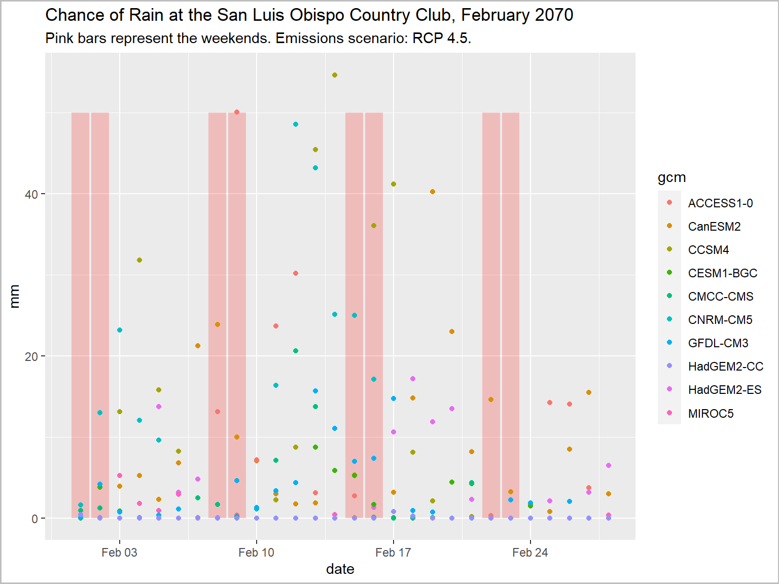
Make this plot
library(caladaptr)
library(dplyr)
library(ggplot2)
library(units)

slo_cap <- ca_loc_pt(coords = c(-120.6276, 35.2130)) %>%
  ca_cvar("pr") %>%
  ca_gcm(gcms[1:10]) %>%
  ca_scenario("rcp45") %>%
  ca_period("day") %>%
  ca_dates(start = "2070-02-01", end = "2070-02-28")

slo_mmday_tbl <- slo_cap %>%
  ca_getvals_tbl(quiet = TRUE) %>%
  mutate(pr_mmday = set_units(as.numeric(val) * 86400, mm/day))

feb2070_weekends_df <- data.frame(dt = as.Date("2070-02-01") + c(0,1,7,8,14,15,21,22), y = 50)

ggplot(data = slo_mmday_tbl, aes(x = as.Date(dt), y = as.numeric(pr_mmday))) +
  geom_col(data = feb2070_weekends_df, aes(x = dt, y = y), fill = "red", alpha = 0.2) +
  geom_point(aes(color=gcm)) +
  labs(title = "Chance of Rain at the San Luis Obispo Country Club, February 2070",
       subtitle = "Pink bars represent the weekends. Emissions scenario: RCP 4.5.",
       x = "date", y = "mm") +
  theme(plot.caption = element_text(hjust = 0))
Best Practices Analyzing Modeled Climate Data
1) Examine 20-30 Year Time Periods
Climate models are designed to capture trends in climate.
By definition, climate is weather averaged over 30+ years.
⇒ If you’re not averaging at least 20-30 years of data, you’re probably doing something wrong.
2) Look at multiple models & emissions scenarios
There is variability among models.
The biggest source of uncertainty (by far) is the future of emissions.
3) Look at both central tendency and the range of variability
Both are important.
Variability can be within and/or between models.
4) Aggregate, aggregate, aggregate
- don’t look at specific points in space or time
- average years together
- average models together
- take rolling averages
- interested in an area? spatially aggregate
5) Compare, compare, compare
- Compare projected future against historical conditions
- Compare Place A vs Place B
- Compare emission scenarios
- Compare models
6) Consider climate analogues
Where can I go right now to see the climate that my city will have 50 years from now?
Comparing the Past to the Future
What is the appropriate historic baseline for modeled future climate scenarios?
Observed historic record and modeled future - different animals
Model historic climate and modeled future - comparable

The Dilemma of Multiple Futures
How do we make sense of multiple climate futures?
How do we store data for multiple futures?
Individual time series are not that helpful by themselves.
What is the right order of operations for computing metrics, aggregating data, and doing comparisons?
Example: How will heat spells in Madera County change under climate change compared to historic conditions?
Source Data (example):
- daily maximum temperature
- 30 years
- 10 GCMs
- 3 emissions scenarios (RCP4.5, RCP8.5, historical)
That’s 365 * 30 * 10 * 3 = 328,500 values of tasmax, for each pixel in the county!
In what order should we
- identify heat days
- find consecutive heat days
- find the mean number of heat spells per i) GCP, ii) RCP, iii) county
General Order of Operations
|
Operation
|
Example
|
R functions
|
- filter by space
|
Madera County, Census tracts, etc.
|
build into API request
|
- filter by year
|
2070-2099
|
build into API request
|
- filter by month or season
|
Sep - June
|
dplyr::filter()
|
- compute daily metrics
|
‘extreme heat’ day
|
dplyr::mutate()
|
- group by emissions scenario
|
RCP
|
dplyr::group_by()
|
- group by time slices
|
water year
|
dplyr::group_by()
|
- group by model
|
GCM
|
dplyr::group_by()
|
- tabluate ‘runs’
|
heat spell = extreme heat for at least 3 days
|
rle()
|
- aggregate / tabulate by model
|
avg # heat spells per GCM (all date slices combined)
|
dplyr::summarise()
|
- aggregate / tabulate by time slice
|
total # heat spells per water year
|
dplyr::summarise()
|
- aggregate / tabulate by scenario
|
avg # heat spells per emissions scenario (all GCMs combined)
|
dplyr::summarise()
|
- compare
|
compare across scenarios, locations
|
plots, tables, stats tests
|
Data Wrangling
Cal-Adapt data always comes down in a “long” format:
ca_loc_pt(coords = c(-117.0, 33.1)) %>%
  ca_cvar(c("tasmax", "tasmin")) %>%
  ca_gcm(gcms[1:4]) %>%
  ca_scenario(scenarios[1:2]) %>%
  ca_period("year") %>%
  ca_years(start = 2040, end = 2060) %>%
  ca_getvals_tbl(quiet = TRUE) %>%
  head()
To make useful plots, maps, and summaries, you often have to ‘munge’ or ‘wrangle’ the data, which may include:
- selecting columns
- filtering rows
- changing column data type
- calculating new columns
- grouping rows; summarizing
- reshaping long to wide (aka pivoting)
Fortunately you have a very robust toolbox:
Top-Seven Data Wrangling Functions
- filter()
- select()
- mutate()
- group_by()
- summarise()
- left_join()
- pivot_wider()
PRO TIP
Qtn. How do I know what data wrangling is needed?
Ans. Work backward from your analysis or visualization functions.
Notebook 2. Find and Wrangle Data
In Notebook 2, you will:
- explore the Cal-Adapt data catalog
- retrieve data using a slug
- wrangle data for visualization and analysis
- make histograms to visualize trends in variability
Notebook 2. Finding Data | solutions
END PART II!