Working with Climate Data in R with caladaptR
February 17, 2022
Andy Lyons

About Me…
About You
Number of registrants: 58
Type of Organization

UC Campus

Familiarity with Climate Change Science

Familiarity with R

Location
Outcomes
1) Get familiar with caladaptR
2) Hands-on practice with:
- importing Cal-Adapt into R via the API
- data wrangling techniques to prep data for visualization or analysis
- see techniques for dealing with large volumes of data
3) Working Code Recipes

+ foundational concepts
+ code recipes
+ working examples
+ practice
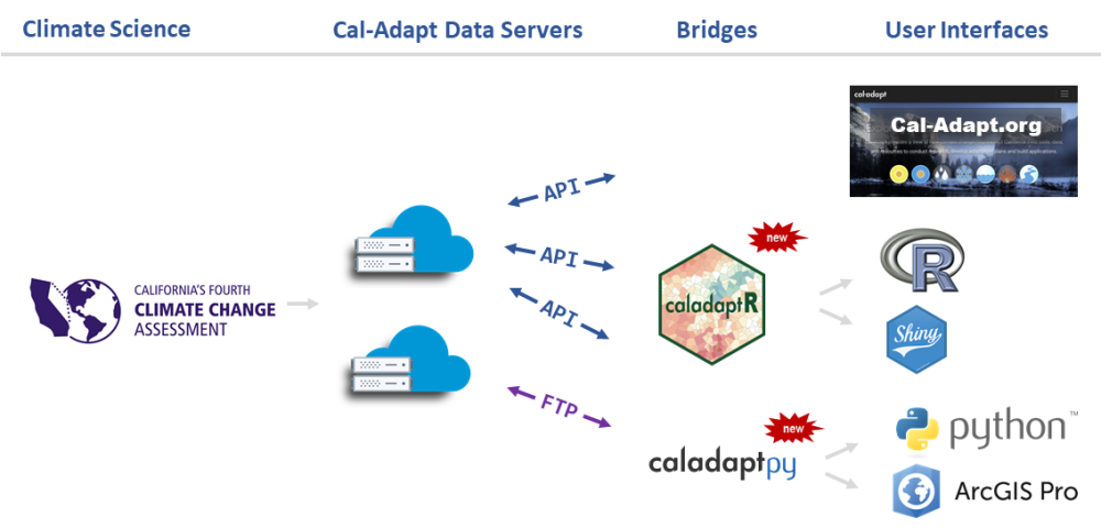
Cal-Adapt
Cal-Adapt is California’s official portal for peer-reviewed climate data.
Datasets are selected with guidance and priorities from California State agencies.
Modeled Climate Data:
- temperature 6 km
- precipitation 6 km
- snow water equivalent 6 km
- relative humidity 6 km
- surface solar radiation 6 km
- wind speed
- wildfire risk
- drought scenarios
- streamflow
- sea level rise
- other derived variables
See also: What climate data does Cal-Adapt provide?.
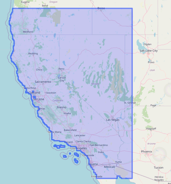
Spatial extent of LOCA downscaled climate data layers:


Where are the Data?
Options for Accessing Cal-Adapt Data
|
Feature
|
Cal-Adapt website
|
Cal-Adapt FTP
|
caladapt-py
|
caladaptR
|
|
Download rasters
|
|
|
|
|
|
Statewide
|
✔
|
✔
|
✔
|
✔
|
|
User area-of-interest
|
✔
|
|
✔
|
✔
|
|
10 recommended GCMs
|
✔
|
✔
|
✔
|
✔
|
|
All 32 GCMs
|
|
✔
|
✔
|
|
|
Query features
|
|
|
|
|
|
Points (user-provided)
|
✔
|
|
✔
|
✔
|
|
Lines (user-provided)
|
✔
|
|
✔
|
|
|
Polygons (user-provided)
|
✔
|
|
✔
|
✔
|
|
Polygons (presets, boundary layers)
|
✔
|
|
|
✔
|
|
Other
|
|
|
|
|
|
Extract underlying tables from preset charts
|
✔
|
|
|
|
More info:
Why you might want to work with Cal-Adapt data in R
Convert statements about climate into actionable info:
The rolling average of maximum daily temperature will increase by X
Species A, B, & C are most likely to survive in the projected climate envelope.
Custom visualizations
Integrate results with other data
- census data
- biodiversity / habitat
- economic data
Take advantage of other R packages
Make your own custom models
caladaptR
Key Features
caladaptr is an API client package
- main job is to provide low-level functions for querying and importing Cal-Adapt data via the API
- uses modern R programming conventions:
- pipe friendly functions
- accepts and returns standard data classes (e.g., tibble, sf, stars)
- units encoded in the results
Main Uses
- Retrieve values from any Cal-Adapt raster series
- Query with user-provided points and polygons
- Query built-in preset areas-of-interest
- Download climate variables as tibbles (data frames) or rasters (tiffs & stars)
Prerequisites
caladaptR users need to know:
- how to work with data in R
- what data you’re looking for
- how to use climate projections wisely
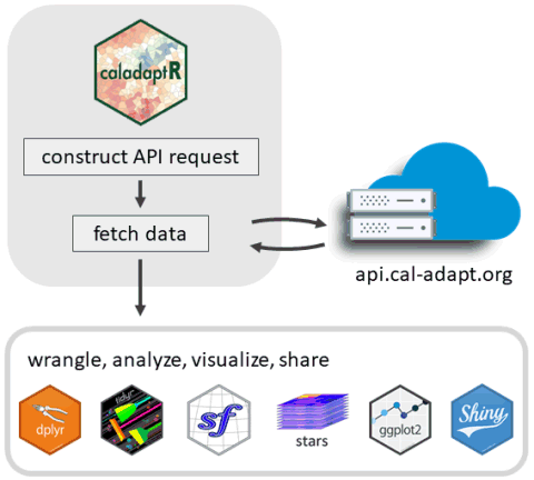
caladaptR workflow
In general, there are five steps to using caladaptR:
Building an API Request
cap1 <- ca_loc_pt(coords = c(-121.4687, 38.5938)) %>%
  ca_cvar(c("tasmax", "tasmin")) %>%
  ca_gcm(gcms[1:4]) %>%
  ca_scenario(scenarios[1:2]) %>%
  ca_period("year") %>%
  ca_years(start = 2040, end = 2060)
An API Request object consists of between 2 and 4 components:
1. Location (required, pick one)
|
ca_loc_aoipreset()
|
Query a preset location(s)
|
|
ca_loc_pt()
|
Question point location(s)
|
|
ca_loc_sf()
|
Query simple feature location(s)
|
2. Raster series dataset
Option 1: Choose downscaled climate projection(s) from Scripps using all 4 of the following constructor functions:
|
ca_cvar()
|
Select the climate variable(s) (i.e., precip, temperature)
|
|
ca_gcm()
|
Pick or more of the 10 Global Climate Models
|
|
ca_period()
|
Select temporal aggregation period (year, month, day)
|
|
ca_scenario()
|
Choose your emission scenario(s)
|
Option 2: Pick any of the 830 raster series datasets by their ‘slug’:
|
ca_slug()
|
Select a dataset by its slug
|
3. Start & end dates (optional, pick one)
|
ca_years()
|
Specify start & end by year
|
|
ca_dates()
|
Specify start & end by date
|
4. Options (only required for polygons)
|
ca_options()
|
Spatial aggregation function(s)
|
Quick Example
- Load the package:
- Create an API request object:
cap1 <- ca_loc_pt(coords = c(-121.4687, 38.5938)) %>%  ## specify a location
  ca_cvar(c("tasmax", "tasmin")) %>%                   ## climate variables
  ca_gcm(gcms[1:4]) %>%                                ## GCM(s)
  ca_scenario(scenarios[1:2]) %>%                      ## emission scenarios(s)
  ca_period("year") %>%                                ## temporal aggregation period
  ca_years(start = 2040, end = 2060)                   ## start and end dates
- Check API request
## Cal-Adapt API Request
## Location(s):
##   x: -121.469
##   y: 38.594
## Variable(s): tasmax, tasmin
## Temporal aggregration period(s): year
## GCM(s): HadGEM2-ES, CNRM-CM5, CanESM2, MIROC5
## Scenario(s): rcp45, rcp85
## Dates: 2040-01-01 to 2060-12-31
##
## General issues
## - none found
## Issues for querying values
## - none found
## Issues for downloading rasters
## - none found
plot(cap1, locagrid = TRUE)
- Fetch data:
cap1_tbl <- ca_getvals_tbl(cap1, quiet = TRUE)
- View the results
R Notebooks
R Notebooks are written in “R Markdown”, which combines text and R code.
Tips
Every time you hit saves, it generates a HTML file in the background.
Remember when you’re in a R Notebook, the working directory is where the Rmd file resides.
Common error:
Error creating notebook: path for html_dependency. Path not found: /tmp/RtmpjR1sPw

- Knit button → Clear Knitr Cache, or
- Restart RStudio
Notebook 1. Getting Started
In Notebook 1, you will:
- Create API requests for i) a point, and ii) a preset area-of-interest (county)
- Wrangle data for plotting
- Plot a time series
Getting Help
- Chat window
- Share screen
- Breakout rooms
Notebook 1. Getting Started | solutions
Other Ways to Specify Location: Preset Areas-of-Interest
The Cal-Adapt API server has 11 preset areas of interest (aka boundary layers).
- Census Tracts
- Counties
- Congressional Districts
- Climatic Regions
- Watersheds
- Irrigated Water Management Districts
- 4th Climate Change Assessment Regions
- Electrical Utilities
- WECC Load Areas
- Event Locations
- Places
You can query these features without passing a spatial object!
Example:
norcal_cap <- ca_loc_aoipreset(type = "counties",
                         idfld = "fips",
                         idval = c("06105", "06049", "06089", "06015")) %>%
  ca_gcm(gcms[1:4]) %>%
  ca_scenario(scenarios[1:2]) %>%
  ca_period("year") %>%
  ca_years(start = 2040, end = 2060) %>%
  ca_cvar("pr") %>%
  ca_options(spatial_ag = "max")
Plot an API request to verify the location:
Other Ways to Specify Location: User-Defined Polygon
An API request can use a simple feature data frame as the query location (point, polygon, and multipolygon).
Use sf::st_read() to import Shapefiles, geojson, KML, geopackage, ESRI geodatabases, etc.
library(sf)
pinnacles_bnd_sf <- st_read("./notebooks/data/pinnacles_bnd.geojson")
## Reading layer `pinnacles_bnd' from data source
##   `D:\GitHub\cal-adapt\caladaptr-res\docs\workshops\ca_intro_feb22\notebooks\data\pinnacles_bnd.geojson'
##   using driver `GeoJSON'
## Simple feature collection with 1 feature and 5 fields
## Geometry type: MULTIPOLYGON
## Dimension:     XY
## Bounding box:  xmin: -121.2455 ymin: 36.4084 xmax: -121.1012 ymax: 36.56416
## Geodetic CRS:  WGS 84
Crate an API request:
pin_cap <- ca_loc_sf(loc = pinnacles_bnd_sf, idfld = "UNIT_CODE") %>%
  ca_slug("et_month_MIROC5_rcp45") %>%
  ca_years(start = 2040, end = 2060) %>%
  ca_options(spatial_ag = "mean")

plot(pin_cap, locagrid = TRUE)
Fetch data:
pin_tbl <- pin_cap %>% ca_getvals_tbl()
head(pin_tbl)
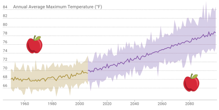
Using Climate Data Wisely
Which weekend in February 2070 has the least chance of rain for my retirement party at the San Luis Obispo Country Club?
Wise or unwise?
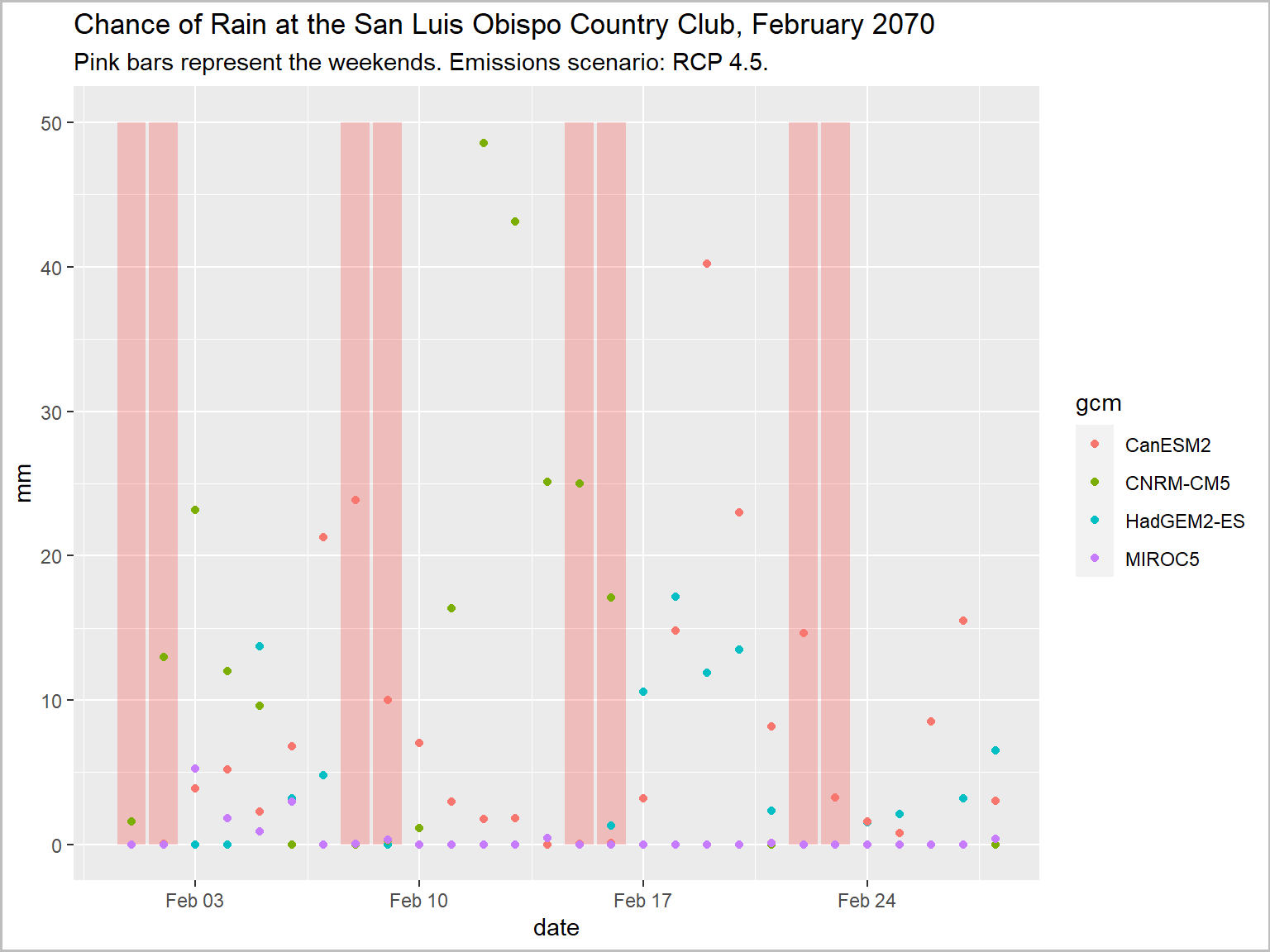
Make this plot
library(caladaptr)
library(dplyr)
library(ggplot2)
library(units)

slo_cap <- ca_loc_pt(coords = c(-120.6276, 35.2130)) %>%
  ca_cvar("pr") %>%
  ca_gcm(gcms[1:4]) %>%
  ca_scenario("rcp45") %>%
  ca_period("day") %>%
  ca_dates(start = "2070-02-01", end = "2070-02-28")

slo_mmday_tbl <- slo_cap %>%
  ca_getvals_tbl(quiet = TRUE) %>%
  mutate(pr_mmday = set_units(as.numeric(val) * 86400, mm/day))

feb2070_weekends_df <- data.frame(dt = as.Date("2070-02-01") + c(0,1,7,8,14,15,21,22), y = 50)

ggplot(data = slo_mmday_tbl, aes(x = as.Date(dt), y = as.numeric(pr_mmday))) +
  geom_col(data = feb2070_weekends_df, aes(x = dt, y = y), fill = "red", alpha = 0.2) +
  geom_point(aes(color=gcm)) +
  labs(title = "Chance of Rain at the San Luis Obispo Country Club, February 2070",
       subtitle = "Pink bars represent the weekends. Emissions scenario: RCP 4.5.",
       x = "date", y = "mm") +
  theme(plot.caption = element_text(hjust = 0))
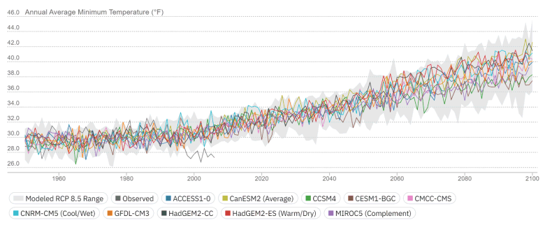
1) Examine 20-30 Year Time Periods
By definition, climate is weather averaged over 30+ years.
Climate models are designed to capture trends in climate.
⇒ If you’re not averaging at least 20-30 years of data, you’re probably doing something wrong.
2) Look at multiple models & emissions scenarios
There is variability among models.
The biggest source of uncertainty (by far) is the future of emissions.
3) Aggregate, aggregate, aggregate
- don’t look at specific points in space or time
- average years together
- average models together
- take rolling averages
- interested in an area? spatially aggregate
4) Look at both central tendency and the range of variability
Both are important.
Variability can be within and/or between models.
4) Compare, compare, compare
- Compare projected future against historical conditions
- Compare Place A vs Place B
- Compare emission scenarios
- Compare models
Climate analogue: Where can I go right now to see the climate that my city will face in 50 years?
How should we compare the past to the future?
Observed historic record and modeled future - different animals
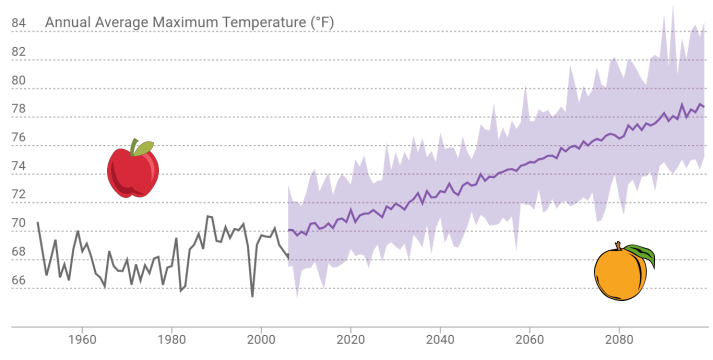
Model historic climate and modeled future - comparable
Raster Series Catalog
caladaptR comes with a Raster Series Catalog
For each raster series the catalog will list its:
- full name
- slug (unique identifier)
- begin and end date
- temporal resolution
- units
- extent
- number of rasters
The catalog can be retrieved using ca_catalog_rs() (returns a tibble).
The best way to browse the catalog is with RStudio’s View pane. You can then use the filter buttons to find the raster series you want.
Data Wrangling
Cal-Adapt data always comes down in a “long” format:
To make useful plots, maps, and summaries, you often have to ‘munge’ or ‘wrangle’ the data, which may include:
- selecting columns
- filtering rows
- changing column data type
- calculating new columns
- grouping rows; summarizing
- reshaping long to wide (aka pivoting)
Fortunately you have a very robust toolbox:
Useful functions
- filter()
- select()
- mutate()
- group_by()
- summarise()
- left_join()
- pivot_wider()
Qtn. How do I know what data wrangling is needed?
Ans. Work backward from your analysis or visualization functions.
Notebook 2. Find and Wrangle Data
In Notebook 2, you will:
- explore the Cal-Adapt data catalog
- retrieve data using a slug
- wrangle data for visualization and analysis
- make histograms to visualize trends in variability
Notebook 2. Finding Data | solutions
Shiny Apps

The Shiny package allows you to create browser-based apps that run R in the background.
You need to know to R, but you don’t need to know JavaScript, HTML, CSS, network protocols, etc.
Can run them locally or online
library(caladaptr.apps)
## Launch the time series app
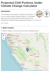
ca_launch("timeseries")
## Launch the projected chill portions app
ca_launch("chill")
Notebook 3. Shiny Apps
In Notebook 3, you will:
- launch a Shiny app using the
caladaptr.apps package
- explore the anatomy of a simple Shiny app
Notebook 3. Shiny Apps
Additional Resources
- documentation
- Articles (tutorials and technical guides)
- R notebooks
- presentations
Work in progress…
- e-book of code recipes
- Degree Day R package
- CA weather APIs
- Shiny apps
Test Cases and Developers Wanted!
- use-cases ⇒ code recipes and Shiny apps
- beta testers
- developers
END!
.png)
.png)
.png)
.png)
.png)

.png)
.png)
.png)
.png)
.png)
.png)
.png)
.png)
.png)