Working with Climate Data in R with caladaptR
October 1, 2021
Andy Lyons
October 1, 2021
Andy Lyons

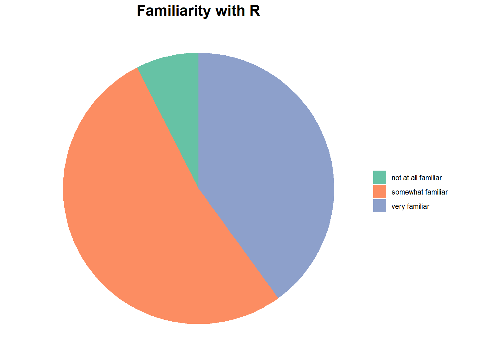
1) Get familiar with caladaptR
2) Hands-on practice with:
3) More caladaptR users!

+ foundational concepts
+ code recipes
+ working examples
+ practice
functional pRoficiency!
Cal-Adapt is California’s official portal for peer-reviewed climate data.
Datasets are selected with guidance and priorities from California State agencies.
Modeled Climate Data:
See also: What climate data does Cal-Adapt provide?.
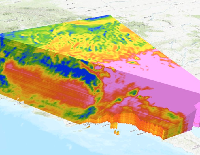
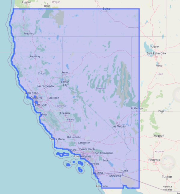
Spatial extent of LOCA downscaled climate data layers:

![]()
![]()
![]()
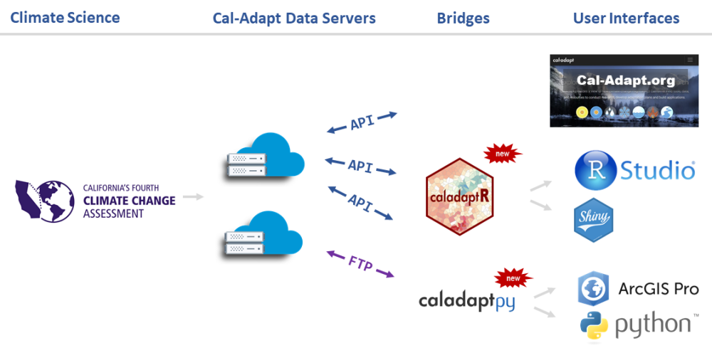
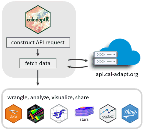
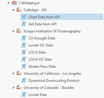
caladaptr is an API client package
caladaptR users need to know:
cap1_tifs <- cap1 %>% ca_getrst_stars(out_dir = “c:/data/tifs”)
ca_read_stars()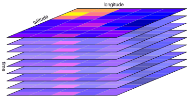
See also Raster Vignettes

Samples:
## Install caladaptr.apps and all dependent packages
remotes::install_github("ucanr-igis/caladaptr.apps")
library(caladaptr.apps)

## Launch the time series app
ca_launch("timeseries")

## Launch the projected chill portions app
ca_launch("chill")R Notebooks are written in “R Markdown”, which combines text and R code.
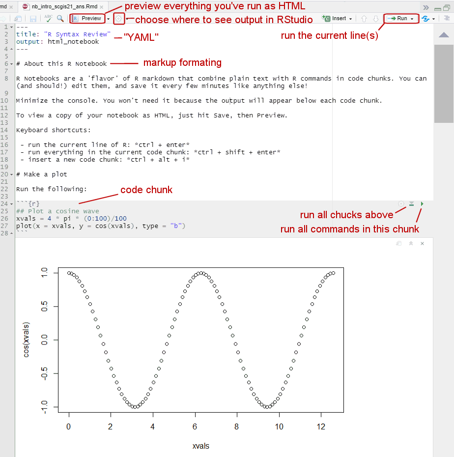
Remember:
When you’re in a R Notebook, the working directory is where the Rmd file resides.