data_dir <- here::here("exercises/data")
dir.exists(data_dir)
[1] TRUEThis Notebook will demonstrate how to:
import weather data from 2023 from a CSV file on disk
compute degree days for a specific model
generate predictions
visualize the predictions as a table and line plot
Most of this code will become the pieces of the online decision support tool.
To compute degree days, the first thing we need is daily temperature data.
For this exercise, we will import some historic data from CIMIS that has already been downloaded, cleaned-up, and saved as CSV (download script). Specifically, we will import temperature data from the Oakville CIMIS station ( Napa County, CA) from 2023.
First, define the data directory:
data_dir <- here::here("exercises/data")
dir.exists(data_dir)[1] TRUENext, define the path to a CSV file containing data from 2023 which has already been imported cleaned:
oakville_fn <- file.path(data_dir, "oakville-cimis-2023.csv")
file.exists(oakville_fn)
[1] TRUEImport with readr:
Rows: 181 Columns: 4
── Column specification ────────────────────────────────────────────────────────
Delimiter: ","
dbl  (3): station_id, tasmin_f, tasmax_f
date (1): dt

ℹ Use `spec()` to retrieve the full column specification for this data.
ℹ Specify the column types or set `show_col_types = FALSE` to quiet this message.head(oakville_tbl)Before you can compute degree days you have to select a degree day model you are computing degree days for. This is because degree days algorithm have specific parameters that must match the prediction model. In other words, there is no “one size fits all” degree day.
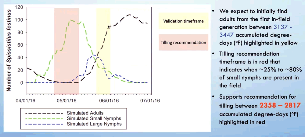
There are many degree models for pests on the UC IPM website. For this exercise, we are using a degree day model developed to inform vineyard managers when to till the soil to disrupt the life cycle of the three-cornered alfalfa hopper (which transmits a disease) (Bick, Kron and Zalom, 2020).

Figure 1. From Kron, 2022

The model provides us seven important parameters:
1. What is being predicted: The recommended window for tilling the soil
2. When to start counting: January 1
3. Method: single sine
4. Lower threshold: 32 degrees F
5. Upper limit: none
6. Cutoff: horizontal
7. Event occurs when: 2358-2817 accumulated degree days (Fahrenheit)
Make sure the temperature units for the lower threshold and the phenology events match the units from the weather data. If you need to convert them, you can use units::set_units().
First, load the dplyr package that we’ll be using to add new columns:
library(dplyr)

# Set preferences for functions with common names
library(conflicted)
conflict_prefer("filter", "dplyr")
conflict_prefer("count", "dplyr")
conflict_prefer("select", "dplyr")
conflict_prefer("arrange", "dplyr")
The degday package has functions for most of the degree day methods. To see what functions it provides, view the documentation.
We can use dd_sng_sine() to compute the daily degree days, and then cumsum() to add them up:
oakville_dd_tbl <- oakville_tbl |>
  mutate(dd_f = dd_sng_sine(daily_min = tasmin_f,
                          daily_max = tasmax_f,
                          thresh_low = 32,
                          thresh_up = 999),
         acc_dd_f = cumsum(dd_f))
- using single sine methodoakville_dd_tblAt this point, you can simply scroll down the accumulated degree day table, and “look up” the dates that fall within our accumulated degree day range (2358-2817).
To find the dates programmatically, we can write a test function that checks to see if the condition has been met:
till_yn <- function(x) {x >= 2358 & x <= 2817}

## Test it:
till_yn(c(2300, 2400, 2500, 2600, 2700, 2800, 2900, 3000))
[1] FALSE TRUE TRUE TRUE TRUE TRUE FALSE FALSENow we use our test function to populate a new column:
View just the days where oakville_till_tbl$till == TRUE:
oakville_till_tbl |> filter(till)To extract just the first and last days:
The same degree day model by Bick et al, 2020 predicts that you can expect to find adults from the first in-field generation between 3137-3447 accumulated degree days (F). Using this model, when would we expect to find adults in 2023? Solution
## Your answer hereA common way to visualize degree day predictions is thru a simple table.
oakville_till_tbl |>
  select(Date = dt, `Min temp (F)` = tasmin_f, `Max temp (F)` = tasmax_f, `Degree Days` = dd_f, `Accumulated DD` = acc_dd_f) |>
knitr::kable()| Date | Min temp (F) | Max temp (F) | Degree Days | Accumulated DD |
|---|---|---|---|---|
| 2023-01-01 | 39.5 | 61.7 | 18.60 | 18.60 |
| 2023-01-02 | 37.7 | 50.5 | 12.10 | 30.70 |
| 2023-01-03 | 41.4 | 49.6 | 13.50 | 44.20 |
| 2023-01-04 | 41.1 | 57.6 | 17.35 | 61.55 |
| 2023-01-05 | 42.9 | 57.0 | 17.95 | 79.50 |
| 2023-01-06 | 45.0 | 57.2 | 19.10 | 98.60 |
| 2023-01-07 | 46.3 | 53.2 | 17.75 | 116.35 |
| 2023-01-08 | 45.8 | 59.2 | 20.50 | 136.85 |
| 2023-01-09 | 41.7 | 60.3 | 19.00 | 155.85 |
| 2023-01-10 | 44.2 | 54.5 | 17.35 | 173.20 |
| 2023-01-11 | 46.4 | 51.7 | 17.05 | 190.25 |
| 2023-01-12 | 47.6 | 63.2 | 23.40 | 213.65 |
| 2023-01-13 | 50.3 | 59.1 | 22.70 | 236.35 |
| 2023-01-14 | 41.2 | 57.1 | 17.15 | 253.50 |
| 2023-01-15 | 40.0 | 53.0 | 14.50 | 268.00 |
| 2023-01-16 | 36.6 | 55.2 | 13.90 | 281.90 |
| 2023-01-17 | 32.6 | 58.9 | 13.75 | 295.65 |
| 2023-01-18 | 32.6 | 51.9 | 10.25 | 305.90 |
| 2023-01-19 | 33.2 | 55.7 | 12.45 | 318.35 |
| 2023-01-20 | 31.5 | 56.7 | 12.13 | 330.48 |
| 2023-01-21 | 28.3 | 59.6 | 12.50 | 342.98 |
| 2023-01-22 | 32.4 | 59.3 | 13.85 | 356.83 |
| 2023-01-23 | 42.6 | 65.8 | 22.20 | 379.03 |
| 2023-01-24 | 37.6 | 66.7 | 20.15 | 399.18 |
| 2023-01-25 | 34.1 | 72.3 | 21.20 | 420.38 |
| 2023-01-26 | 40.0 | 73.0 | 24.50 | 444.88 |
| 2023-01-27 | 34.0 | 61.8 | 15.90 | 460.78 |
| 2023-01-28 | 29.5 | 58.2 | 12.17 | 472.95 |
| 2023-01-29 | 34.1 | 49.5 | 9.80 | 482.75 |
| 2023-01-30 | 36.1 | 56.9 | 14.50 | 497.25 |
| 2023-01-31 | 32.6 | 59.4 | 14.00 | 511.25 |
| 2023-02-01 | 29.7 | 59.2 | 12.72 | 523.97 |
| 2023-02-02 | 32.3 | 58.7 | 13.50 | 537.47 |
| 2023-02-03 | 42.0 | 54.6 | 16.30 | 553.77 |
| 2023-02-04 | 44.5 | 57.1 | 18.80 | 572.57 |
| 2023-02-05 | 37.5 | 54.5 | 14.00 | 586.57 |
| 2023-02-06 | 31.9 | 65.1 | 16.50 | 603.07 |
| 2023-02-07 | 32.8 | 62.0 | 15.40 | 618.47 |
| 2023-02-08 | 33.2 | 66.2 | 17.70 | 636.17 |
| 2023-02-09 | 34.2 | 66.6 | 18.40 | 654.57 |
| 2023-02-10 | 31.9 | 60.4 | 14.15 | 668.72 |
| 2023-02-11 | 37.1 | 60.1 | 16.60 | 685.32 |
| 2023-02-12 | 36.0 | 73.6 | 22.80 | 708.12 |
| 2023-02-13 | 33.7 | 68.2 | 18.95 | 727.07 |
| 2023-02-14 | 31.0 | 53.7 | 10.44 | 737.51 |
| 2023-02-15 | 32.1 | 62.3 | 15.20 | 752.71 |
| 2023-02-16 | 28.7 | 55.1 | 10.40 | 763.11 |
| 2023-02-17 | 33.9 | 64.1 | 17.00 | 780.11 |
| 2023-02-18 | 28.8 | 64.7 | 15.16 | 795.27 |
| 2023-02-19 | 31.1 | 67.5 | 17.36 | 812.63 |
| 2023-02-20 | 35.0 | 69.7 | 20.35 | 832.98 |
| 2023-02-21 | 36.3 | 64.4 | 18.35 | 851.33 |
| 2023-02-22 | 30.8 | 52.5 | 9.77 | 861.10 |
| 2023-02-23 | 26.2 | 48.6 | 6.69 | 867.79 |
| 2023-02-24 | 33.1 | 49.0 | 9.05 | 876.84 |
| 2023-02-25 | 36.4 | 48.7 | 10.55 | 887.39 |
| 2023-02-26 | 34.8 | 49.0 | 9.90 | 897.29 |
| 2023-02-27 | 31.0 | 49.3 | 8.25 | 905.54 |
| 2023-02-28 | 33.5 | 53.0 | 11.25 | 916.79 |
| 2023-03-01 | 29.8 | 55.5 | 10.93 | 927.72 |
| 2023-03-02 | 33.1 | 61.4 | 15.25 | 942.97 |
| 2023-03-03 | 31.5 | 60.8 | 14.18 | 957.15 |
| 2023-03-04 | 37.7 | 52.3 | 13.00 | 970.15 |
| 2023-03-05 | 33.0 | 51.7 | 10.35 | 980.50 |
| 2023-03-06 | 33.2 | 53.0 | 11.10 | 991.60 |
| 2023-03-07 | 33.2 | 52.8 | 11.00 | 1002.60 |
| 2023-03-08 | 35.9 | 57.1 | 14.50 | 1017.10 |
| 2023-03-09 | 34.0 | 53.2 | 11.60 | 1028.70 |
| 2023-03-10 | 43.7 | 58.5 | 19.10 | 1047.80 |
| 2023-03-11 | 41.1 | 54.0 | 15.55 | 1063.35 |
| 2023-03-12 | 51.3 | 57.1 | 22.20 | 1085.55 |
| 2023-03-13 | 53.2 | 60.5 | 24.85 | 1110.40 |
| 2023-03-14 | 41.0 | 58.9 | 17.95 | 1128.35 |
| 2023-03-15 | 35.1 | 65.9 | 18.50 | 1146.85 |
| 2023-03-16 | 34.3 | 65.8 | 18.05 | 1164.90 |
| 2023-03-17 | 36.0 | 68.1 | 20.05 | 1184.95 |
| 2023-03-18 | 39.1 | 65.4 | 20.25 | 1205.20 |
| 2023-03-19 | 48.9 | 55.5 | 20.20 | 1225.40 |
| 2023-03-20 | 40.6 | 59.5 | 18.05 | 1243.45 |
| 2023-03-21 | 43.3 | 50.2 | 14.75 | 1258.20 |
| 2023-03-22 | 44.7 | 56.8 | 18.75 | 1276.95 |
| 2023-03-23 | 38.9 | 60.3 | 17.60 | 1294.55 |
| 2023-03-24 | 33.7 | 59.6 | 14.65 | 1309.20 |
| 2023-03-25 | 32.7 | 61.0 | 14.85 | 1324.05 |
| 2023-03-26 | 31.2 | 60.1 | 13.71 | 1337.76 |
| 2023-03-27 | 28.8 | 63.2 | 14.42 | 1352.18 |
| 2023-03-28 | 40.1 | 51.9 | 14.00 | 1366.18 |
| 2023-03-29 | 41.3 | 47.5 | 12.40 | 1378.58 |
| 2023-03-30 | 34.8 | 60.5 | 15.65 | 1394.23 |
| 2023-03-31 | 34.7 | 60.5 | 15.60 | 1409.83 |
| 2023-04-01 | 35.0 | 62.9 | 16.95 | 1426.78 |
| 2023-04-02 | 40.0 | 61.9 | 18.95 | 1445.73 |
| 2023-04-03 | 33.9 | 59.1 | 14.50 | 1460.23 |
| 2023-04-04 | 33.2 | 60.5 | 14.85 | 1475.08 |
| 2023-04-05 | 34.0 | 62.3 | 16.15 | 1491.23 |
| 2023-04-06 | 35.6 | 64.7 | 18.15 | 1509.38 |
| 2023-04-07 | 46.9 | 61.1 | 22.00 | 1531.38 |
| 2023-04-08 | 42.5 | 67.7 | 23.10 | 1554.48 |
| 2023-04-09 | 39.1 | 75.9 | 25.50 | 1579.98 |
| 2023-04-10 | 44.2 | 76.9 | 28.55 | 1608.53 |
| 2023-04-11 | 45.5 | 70.6 | 26.05 | 1634.58 |
| 2023-04-12 | 37.0 | 66.6 | 19.80 | 1654.38 |
| 2023-04-13 | 41.5 | 69.5 | 23.50 | 1677.88 |
| 2023-04-14 | 35.5 | 67.3 | 19.40 | 1697.28 |
| 2023-04-15 | 38.1 | 68.6 | 21.35 | 1718.63 |
| 2023-04-16 | 36.8 | 68.9 | 20.85 | 1739.48 |
| 2023-04-17 | 40.4 | 62.6 | 19.50 | 1758.98 |
| 2023-04-18 | 36.8 | 60.4 | 16.60 | 1775.58 |
| 2023-04-19 | 35.8 | 66.8 | 19.30 | 1794.88 |
| 2023-04-20 | 38.2 | 74.0 | 24.10 | 1818.98 |
| 2023-04-21 | 47.3 | 83.9 | 33.60 | 1852.58 |
| 2023-04-22 | 47.3 | 84.3 | 33.80 | 1886.38 |
| 2023-04-23 | 49.5 | 80.4 | 32.95 | 1919.33 |
| 2023-04-24 | 43.0 | 77.0 | 28.00 | 1947.33 |
| 2023-04-25 | 41.2 | 85.4 | 31.30 | 1978.63 |
| 2023-04-26 | 43.0 | 87.4 | 33.20 | 2011.83 |
| 2023-04-27 | 47.3 | 91.2 | 37.25 | 2049.08 |
| 2023-04-28 | 49.0 | 86.6 | 35.80 | 2084.88 |
| 2023-04-29 | 45.4 | 77.9 | 29.65 | 2114.53 |
| 2023-04-30 | 40.8 | 73.9 | 25.35 | 2139.88 |
| 2023-05-01 | 46.7 | 58.5 | 20.60 | 2160.48 |
| 2023-05-02 | 46.9 | 57.4 | 20.15 | 2180.63 |
| 2023-05-03 | 44.8 | 61.7 | 21.25 | 2201.88 |
| 2023-05-04 | 41.9 | 60.7 | 19.30 | 2221.18 |
| 2023-05-05 | 44.0 | 61.7 | 20.85 | 2242.03 |
| 2023-05-06 | 42.9 | 64.6 | 21.75 | 2263.78 |
| 2023-05-07 | 38.9 | 65.7 | 20.30 | 2284.08 |
| 2023-05-08 | 46.0 | 66.1 | 24.05 | 2308.13 |
| 2023-05-09 | 43.2 | 70.6 | 24.90 | 2333.03 |
| 2023-05-10 | 40.9 | 69.7 | 23.30 | 2356.33 |
| 2023-05-11 | 41.5 | 75.3 | 26.40 | 2382.73 |
| 2023-05-12 | 44.6 | 79.6 | 30.10 | 2412.83 |
| 2023-05-13 | 47.3 | 92.0 | 37.65 | 2450.48 |
| 2023-05-14 | 51.2 | 74.8 | 31.00 | 2481.48 |
| 2023-05-15 | 46.3 | 80.6 | 31.45 | 2512.93 |
| 2023-05-16 | 46.5 | 90.4 | 36.45 | 2549.38 |
| 2023-05-17 | 47.3 | 83.1 | 33.20 | 2582.58 |
| 2023-05-18 | 45.9 | 77.6 | 29.75 | 2612.33 |
| 2023-05-19 | 46.2 | 77.1 | 29.65 | 2641.98 |
| 2023-05-20 | 46.0 | 75.3 | 28.65 | 2670.63 |
| 2023-05-21 | 51.2 | 78.9 | 33.05 | 2703.68 |
| 2023-05-22 | 50.5 | 84.2 | 35.35 | 2739.03 |
| 2023-05-23 | 50.7 | 70.6 | 28.65 | 2767.68 |
| 2023-05-24 | 48.3 | 71.2 | 27.75 | 2795.43 |
| 2023-05-25 | 48.7 | 70.0 | 27.35 | 2822.78 |
| 2023-05-26 | 51.2 | 68.8 | 28.00 | 2850.78 |
| 2023-05-27 | 51.5 | 73.0 | 30.25 | 2881.03 |
| 2023-05-28 | 51.4 | 69.2 | 28.30 | 2909.33 |
| 2023-05-29 | 48.1 | 66.2 | 25.15 | 2934.48 |
| 2023-05-30 | 46.6 | 67.0 | 24.80 | 2959.28 |
| 2023-05-31 | 51.5 | 72.4 | 29.95 | 2989.23 |
| 2023-06-01 | 48.4 | 75.0 | 29.70 | 3018.93 |
| 2023-06-02 | 46.6 | 80.7 | 31.65 | 3050.58 |
| 2023-06-03 | 47.2 | 87.6 | 35.40 | 3085.98 |
| 2023-06-04 | 47.2 | 82.0 | 32.60 | 3118.58 |
| 2023-06-05 | 52.8 | 77.0 | 32.90 | 3151.48 |
| 2023-06-06 | 54.5 | 70.2 | 30.35 | 3181.83 |
| 2023-06-07 | 52.8 | 65.7 | 27.25 | 3209.08 |
| 2023-06-08 | 51.9 | 78.8 | 33.35 | 3242.43 |
| 2023-06-09 | 50.9 | 74.4 | 30.65 | 3273.08 |
| 2023-06-10 | 48.3 | 75.3 | 29.80 | 3302.88 |
| 2023-06-11 | 50.2 | 73.0 | 29.60 | 3332.48 |
| 2023-06-12 | 54.2 | 74.6 | 32.40 | 3364.88 |
| 2023-06-13 | 53.3 | 78.4 | 33.85 | 3398.73 |
| 2023-06-14 | 49.9 | 75.3 | 30.60 | 3429.33 |
| 2023-06-15 | 52.4 | 79.9 | 34.15 | 3463.48 |
| 2023-06-16 | 46.6 | 79.6 | 31.10 | 3494.58 |
| 2023-06-17 | 49.4 | 79.3 | 32.35 | 3526.93 |
| 2023-06-18 | 48.3 | 83.8 | 34.05 | 3560.98 |
| 2023-06-19 | 42.4 | 76.1 | 27.25 | 3588.23 |
| 2023-06-20 | 44.8 | 77.8 | 29.30 | 3617.53 |
| 2023-06-21 | 42.4 | 83.4 | 30.90 | 3648.43 |
| 2023-06-22 | 44.0 | 74.2 | 27.10 | 3675.53 |
| 2023-06-23 | 49.6 | 75.2 | 30.40 | 3705.93 |
| 2023-06-24 | 46.2 | 78.4 | 30.30 | 3736.23 |
| 2023-06-25 | 48.4 | 75.0 | 29.70 | 3765.93 |
| 2023-06-26 | 51.3 | 75.4 | 31.35 | 3797.28 |
| 2023-06-27 | 48.0 | 74.0 | 29.00 | 3826.28 |
| 2023-06-28 | 50.8 | 76.0 | 31.40 | 3857.68 |
| 2023-06-29 | 48.7 | 89.7 | 37.20 | 3894.88 |
| 2023-06-30 | 50.1 | 95.5 | 40.80 | 3935.68 |
The DT (DataTables) package provides R functions to create interactive HTML tables, which may be more suitable for an online decision support tool.
Basic usage:
library(DT)

oakville_till4dt_tbl <- oakville_till_tbl |>
  # filter(month(dt) == 5) |>
  select(dt, tasmin_f, tasmax_f, dd_f, acc_dd_f, till)

DT::datatable(oakville_till4dt_tbl |> select(-till),
              colnames = c("Date", "Min temp", "Max temp", "Deg Day", "Accum DD"),
              caption = "Recommended Days to Till, Oakville",
              rownames = FALSE,
              autoHideNavigation = FALSE,
              escape =FALSE,
              options = list(pageLength = 8,
                             searching = FALSE,
                             info = FALSE))
You can add formatStyle() to apply conditional formatting to specific rows:
till_rows_idx <- which(oakville_till4dt_tbl$till)

DT::datatable(oakville_till4dt_tbl |> select(-till),
              colnames = c("Date", "Min temp", "Max temp", "Deg Day", "Accum DD"),
              caption = "Recommended Days to Till, Oakville",
              rownames = FALSE,
              autoHideNavigation = FALSE,
              escape =FALSE,
              options = list(pageLength = 15,
                             searching = FALSE,
                             info = FALSE)) |>
  formatStyle(columns = 0,
              target = "row",
              color = styleRow(till_rows_idx, "red"),
              backgroundColor = styleRow(till_rows_idx, "#eee"),
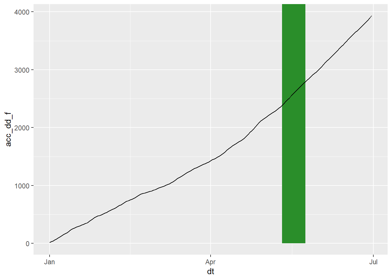
fontWeight = styleRow(till_rows_idx, "bold"))Plots are often a better way to visualize time series data. We start by creating a simple ggplot of the accumulated degree days:
Add a shaded region for the recommended tilling window:
oakville_till_tbl |> filter(till) |> pull(dt) |> range() -> till_dates

ggplot(oakville_till_tbl, mapping = aes(x = dt, y = acc_dd_f)) +
  geom_rect(aes(xmin = till_dates[1], xmax = till_dates[2],
                ymin = 0, ymax =Inf),
            fill = 'darkgreen', alpha = 0.01) +
  geom_line()
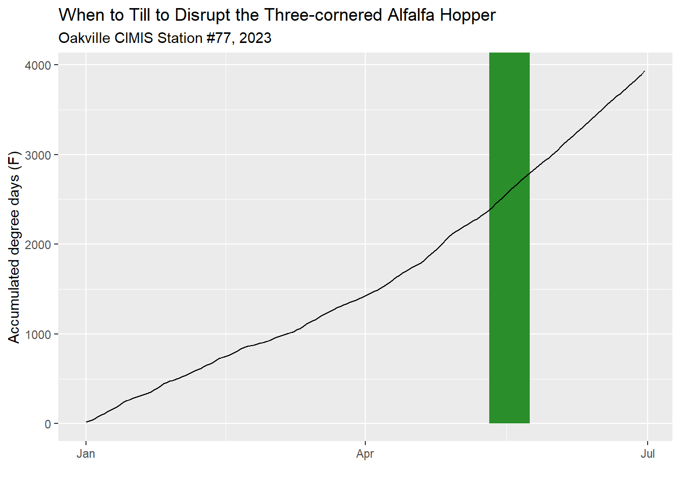
Finally, add some labels:
ggplot(oakville_till_tbl, mapping = aes(x = dt, y = acc_dd_f)) +
  geom_rect(aes(xmin = till_dates[1], xmax = till_dates[2],
                ymin = 0, ymax =Inf),
            fill = 'darkgreen', alpha = 0.01) +
  geom_line() +
  labs(title = "When to Till to Disrupt the Three-cornered Alfalfa Hopper",
       subtitle = "Oakville CIMIS Station #77, 2023") +
  xlab("") +
  ylab("Accumulated degree days (F)")
Identify the best time to till in 2023 using data from the Santa Rosa CIMIS Station (see santarosa-cimis-2023.csv)