Exercise 3: Download the Short-Term and Seasonal Forecasts

Summary

This Notebook demonstrates how to get for one location:

1. 7-day the short-term forecast (Open-Meteo)
   
2. 90-day seasonal forecast (Open-Meteo)
   
3. 30-year historic daily averages (gridMet, Cal-Adapt)

Our desired output are tables with the following columns:

• loc_id: location id
  
• period: “recnt” (recent past) | “stf” (short term forecast) | “hist_avg” (historic average) | “ssnfcast” (seasonal forecast)
• date: date
  
• tasmin: minimum daily temperature
  
• tasmax: maximum daily temperature

1 Short-Term Forecast

For the first part of this Notebook, we’ll be using an API service from Open-Meteo. The first thing you should always do is read about the data.

Highlights:

• Open-Meteo’s brings together numerous weather forecast models from national weather services.

• API queries are sampled from modeled rasters with resolutions ranging from 1 - 11km , not stations (i.e., you query locations based on coordinates).

• In addition to the 7-day forecast, they have APIs for historic weather, seasonal forecast, ensemble models, air quality, etc.

• Data are available at both hourly and daily temporal resolution

• They have both paid and free plans (for non-commercial use)

2 Gather all the information needed to query the API

2.1 1. Generate an API token

An API token is not needed for Open-Meteo.

2.2 2. Define the location of interest

The Open-Meteo API requires locations to be expressed by longitude and latitude coordinates.

The longitude and latitude for CIMIS Station 077 (Oakville) is:

stn_coords <- c(-122.410, 38.434)

2.3 3. Determine which Weather Forecast / model end point to use

https://open-meteo.com/en/docs

We will use the US NOAA GFS weather model. More info at:

https://open-meteo.com/en/docs/gfs-api

2.4 4. Load the openmeteo R package

Fortunately, Tom Pisel has already written a R package for the Open-Meteo API, openmeteo:

library(openmeteo)

openmeteo has functions to call Open-Meteo’s weather forecast and historical weather APIs.

Read about the arguments for weather_forecast().

# help(weather_forecast)

2.5 5. Define the daily weather variables we want

weather_variables() provides a list of the most common weather variables:

om_vars_lst <- weather_variables()

om_vars_lst$daily_forecast_vars

 [1] "temperature_2m_max"          "temperature_2m_min"         
 [3] "apparent_temperature_max"    "apparent_temperature_min"   
 [5] "precipitation_sum"           "precipitation_hours"        
 [7] "weather_code"                "sunrise"                    
 [9] "sunset"                      "wind_speed_10m_max"         
[11] "wind_gusts_10m_max"          "wind_direction_10m_dominant"
[13] "shortwave_radiation_sum"     "uv_index_max"               
[15] "uv_index_clear_sky_max"      "et0_fao_evapotranspiration" 

We will use the following:

om_weather_vars <- c("temperature_2m_min", "temperature_2m_max")

2.6 6. Define the start and end dates:

start_date <- Sys.Date()
end_date <- Sys.Date() + 7

start_date; end_date

[1] "2024-05-22"

[1] "2024-05-29"

2.7 7. Call the API

We now have everything we need to call the API using weather_forecast():

# Load a cached copy
om_forecast_dly_tbl <- readRDS(here::here("exercises/cached_api_responses/ex03_om_forecast_dly_tbl.Rds"))

# If you really want to send the request, uncomment the following:
# om_forecast_dly_tbl <- weather_forecast(
#   location = stn_coords[c(2,1)],
#   start = start_date,
#   end = end_date,
#   daily = om_weather_vars,
#   response_units = list(temperature_unit = "fahrenheit"),
#   timezone = "America/Los_Angeles"
# )
# saveRDS(om_forecast_dly_tbl, here::here("exercises/cached_api_responses/ex03_om_forecast_dly_tbl.Rds"))

om_forecast_dly_tbl

2.8 8. Prepare the final tibble:

Load dplyr and set conflict preferences:

library(dplyr) |> suppressPackageStartupMessages()

# Set preferences for functions with common names 
library(conflicted)
conflict_prefer("filter", "dplyr", quiet = TRUE)
conflict_prefer("count", "dplyr", quiet = TRUE)
conflict_prefer("select", "dplyr", quiet = TRUE)
conflict_prefer("arrange", "dplyr", quiet = TRUE)

Add required columns:

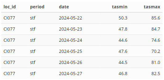
stn_shrtfrcst_dlytas_tbl <- om_forecast_dly_tbl |> 
  mutate(loc_id = "CI077", period = "stf") |> 
  select(loc_id, period, date, tasmin = daily_temperature_2m_min, tasmax = daily_temperature_2m_max)

stn_shrtfrcst_dlytas_tbl

Save the table to disk for use in the next exercise:

saveRDS(stn_shrtfrcst_dlytas_tbl,
        file = here::here("exercises/data/stn_shrtfrcst_dlytas_tbl.Rds"))

3 Seasonal Forecast

Sometimes degree day model predictions may be several weeks out. If you want to provide estimated degree days for the rest of the season (which are admittedly less accurate), you can use a seasonal forecast or historic daily averages as the best guess for the rest of the season.

The openmeteo package does not have a function to call the Seasonal Forecast end point, so we will have to call it and process the response using httr2.

3.1 Define the base URL

om_ssnfcast_base <- "https://seasonal-api.open-meteo.com/v1/seasonal"

3.2 Define the start and end dates

ssnfcast_start_date <- Sys.Date() + 8
ssnfcast_start_date

[1] "2024-05-30"

ssnfcast_end_date <- ssnfcast_start_date + 90
ssnfcast_end_date

[1] "2024-08-28"

3.3 Define the daily weather variables we need

We want the following:

om_weather_vars <- c("temperature_2m_min", "temperature_2m_max")

3.4 Create the API Request Object

library(httr2)

om_ssnfcast_req <- request(om_ssnfcast_base) |> 
  req_headers("Accept" = "application/json") |> 
  req_url_query(latitude = stn_coords[2], 
                longitude = stn_coords[1],
                start_date = format(ssnfcast_start_date, "%Y-%m-%d"),
                end_date = format(ssnfcast_end_date, "%Y-%m-%d"),
                daily = om_weather_vars,
                temperature_unit = "fahrenheit",
                timezone = "America/Los_Angeles",
                .multi = "comma") 

om_ssnfcast_req

<httr2_request>

GET
https://seasonal-api.open-meteo.com/v1/seasonal?latitude=38.434&longitude=-122.41&start_date=2024-05-30&end_date=2024-08-28&daily=temperature_2m_min,temperature_2m_max&temperature_unit=fahrenheit&timezone=America%2FLos_Angeles

Headers:

• Accept: 'application/json'

Body: empty

3.5 Send the request

# Load a cached copy
om_ssnfcast_resp <- readRDS(here::here("exercises/cached_api_responses/ex03_om_ssnfcast_resp.Rds"))

# If you really want to send the request, uncomment the following:
# om_ssnfcast_resp <- om_ssnfcast_req |> req_perform()
# saveRDS(om_ssnfcast_resp, here::here("exercises/cached_api_responses/ex03_om_ssnfcast_resp.Rds"))

om_ssnfcast_resp

<httr2_response>

GET
https://seasonal-api.open-meteo.com/v1/seasonal?latitude=38.434&longitude=-122.41&start_date=2024-05-30&end_date=2024-08-28&daily=temperature_2m_min,temperature_2m_max&temperature_unit=fahrenheit&timezone=America%2FLos_Angeles

Status: 200 OK

Content-Type: application/json

Body: In memory (5592 bytes)

3.6 Convert the response body to a list

om_ssnfcast_lst <- om_ssnfcast_resp |> resp_body_json()

# View(om_ssnfcast_lst)

3.7 Extract the values

library(lubridate)
library(purrr)

om_ssnfcast_tbl <- tibble(
  date = om_ssnfcast_lst$daily$time |> unlist() |> ymd(),
  tasmin = om_ssnfcast_lst$daily$temperature_2m_min_member01 |> modify_if(is_null, ~NA) |> unlist(),
  tasmax = om_ssnfcast_lst$daily$temperature_2m_max_member01 |> modify_if(is_null, ~NA) |> unlist()
)

head(om_ssnfcast_tbl)

# om_ssnfcast_tbl |> View()

3.8 Create the final table

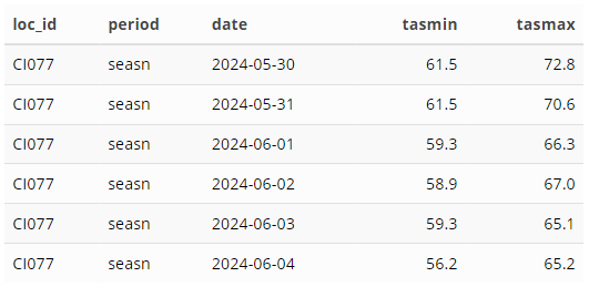
stn_ssnfcast_dlytas_tbl <- om_ssnfcast_tbl |> 
  mutate(loc_id = "CI077", period = "seasn") |> 
  select(loc_id, period, date, tasmin, tasmax)

stn_ssnfcast_dlytas_tbl

Save the final table to disk:

saveRDS(stn_ssnfcast_dlytas_tbl,
        file = here::here("exercises/data/stn_ssnfcast_dlytas_tbl.Rds"))

4 Computing the Daily Historic Averages as Proxy for the Seasonal Forecast

Another commonly used proxy for the seasonal forecast are the historic daily averages.

Some good practices:

• compute daily averages from at least 30 years of data
  
• using modeled data is preferable to simply averaging measurements (which are prone to noise and extreme events)

In this section, we’ll use 30-years of gridMet data imported from Cal-Adapt using caladaptR.

library(caladaptr)

caladaptr (version 0.6.8)
URL: https://ucanr-igis.github.io/caladaptr
Bug reports: https://github.com/ucanr-igis/caladaptr/issues

4.1 Find the gridMet datasets

The first step is to identify the ‘slug’ of the gridMet datasets for daily minimum and maximum temperatures:

## View the entire catalog in a View window
## ca_catalog_rs() |> View()

Next, we can preview the metadata for the gridMet daily temperatures:

ca_catalog_search("tmmn_day_gridmet")

tmmn_day_gridmet

  name: gridMET daily minimum temperature historical

  url: https://api.cal-adapt.org/api/series/tmmn_day_gridmet/

  tres: daily

  begin: 1979-01-01T00:00:00Z

  end: 2020-12-31T00:00:00Z

  units: K

  num_rast: 1

  id: 919

  xmin: -124.579167

  xmax: -113.370833

  ymin: 31.545833

  ymax: 43.754167

ca_catalog_search("tmmx_day_gridmet")

tmmx_day_gridmet

  name: gridMET daily maximum temperature historical

  url: https://api.cal-adapt.org/api/series/tmmx_day_gridmet/

  tres: daily

  begin: 1979-01-01T00:00:00Z

  end: 2020-12-31T00:00:00Z

  units: K

  num_rast: 1

  id: 921

  xmin: -124.579167

  xmax: -113.370833

  ymin: 31.545833

  ymax: 43.754167

4.2 Create the request object

stn_coords <- c(-122.410, 38.434)

stn_hist_tas_cap <- ca_loc_pt(coords = stn_coords) |> 
  ca_years(start = 1990, end = 2020) |> 
  ca_slug(c("tmmn_day_gridmet", "tmmx_day_gridmet"))

stn_hist_tas_cap

Cal-Adapt API Request
Location(s): 
  x: -122.41
  y: 38.434
Slug(s): tmmn_day_gridmet, tmmx_day_gridmet
Dates: 1990-01-01 to 2020-12-31
 

4.3 Query the API

First we can do a pre-flight check:

stn_hist_tas_cap |> ca_preflight()

General issues
 - none found
Issues for querying values
 - none found
Issues for downloading rasters
 - none found

Next, fetch the data:

## Load a cached copy
stn_hist_tas_tbl <- readRDS(here::here("exercises/cached_api_responses/ex03_stn_hist_tas_tbl.Rds"))

# If you really want to send the request, uncomment the following:
# stn_hist_tas_tbl <- stn_hist_tas_cap |> ca_getvals_tbl()
# saveRDS(stn_hist_tas_tbl, here::here("exercises/cached_api_responses/ex03_stn_hist_tas_tbl.Rds"))

Inspect the results:

dim(stn_hist_tas_tbl)

[1] 22646     5

head(stn_hist_tas_tbl)

stn_hist_tas_tbl$dt |> range()

[1] "1990-01-01" "2020-12-31"

4.4 Wrangle the data

We now have to transform 30-years of daily data into estimates of daily temperature values for the rest of the current season. This will involve:

1. Computing the Julian days for the historic data
   
2. Using the Julian days to filter the days-of-the-year we want
   
3. Grouping the data by Julian day
   
4. Taking the average minimum and maximum daily temperatures
   
5. Converting the units from Kelvin to Fahrenheit
   
6. Reshaping the data from long to wide
   
7. Converting the Julian numbers to future dates for the current season
8. Renaming the columns to match the desired template

First, we define the start and end dates, and get their Julian day numbers.

library(lubridate)

ssnfcast_start_date <- Sys.Date() + 8
ssnfcast_end_date <- ssnfcast_start_date + 90

ssnfcast_start_date

[1] "2024-05-30"

ssnfcast_end_date

[1] "2024-08-28"

Next, get their Julian date numbers:

ssnfcast_start_yday <- yday(ssnfcast_start_date)
ssnfcast_end_yday <- yday(ssnfcast_end_date) 

ssnfcast_start_yday

[1] 151

ssnfcast_end_yday

[1] 241

We now have everything we need to wrangle the data. We need to load a couple more packages:

library(tidyr)
library(units)

udunits database from C:/Users/Andy/AppData/Local/R/win-library/4.4/units/share/udunits/udunits2.xml

Putting the tidyverse to work:

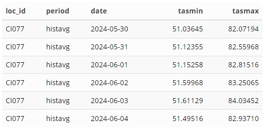
stn_histavg_dlytas_tbl <- stn_hist_tas_tbl |> 
  mutate(dt_yday = yday(dt)) |> 
  filter(dt_yday >= ssnfcast_start_yday, dt_yday <= ssnfcast_end_yday) |> 
  group_by(dt_yday, slug) |> 
  summarize(avg_tempK = mean(val), .groups = "drop") |> 
  mutate(avg_tempF = set_units(avg_tempK, degF)) |> 
  pivot_wider(id_cols= dt_yday, names_from = slug, values_from = avg_tempF) |> 
  mutate(loc_id = "CI077",
         period = "histavg",
         date = make_date(year = 2024, month = 1, day = 1) + dt_yday - 1,
         tasmin = as.numeric(tmmn_day_gridmet),
         tasmax = as.numeric(tmmx_day_gridmet)) |> 
  select(loc_id, period, date, tasmin, tasmax)
  
stn_histavg_dlytas_tbl

Save the final table to disk:

saveRDS(stn_histavg_dlytas_tbl,
        file = here::here("exercises/data/stn_histavg_dlytas_tbl.Rds"))