Spatial Data Analysis with R
Society for Conservation GIS, July 2021

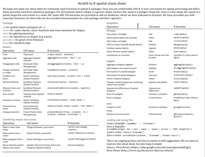
Connecting R and ArcGIS

Cross-Walking R and ArcGIS Pro

ArcGIS to R spatial cheatsheet

R-ArcGIS Bridge

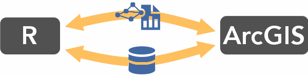
The R-ArcGIS Bridge is a R package that allows you to exchange spatial data between R and ArcGIS Pro / ArcGIS.com.

Installation

Requires a licensed copy of ArcGIS Pro installed

Install the package from within ArcGIS Pro

Close RStudio
ArcGIS Pro >> Project >> Options >> Geoprocessing >> R-ArcGIS Support
Open RStudio
library(arcgisbinding)

Instructions for ArcMap users here.

What You Can Do with the R-ArcGIS Bridge

View spatial metadata before importing data into R.
Import spatial layers (both vector and raster) from geodatabases, Shapefiles, etc.
Import spatial data from ArcGIS.com and ArcGIS Enterprise servers.
Create R scripts that you run from ArcGIS toolboxes.

The R-ArcGIS Bridge is primarily for programatically transferring spatial data between R and ArcGIS.

It does not have all the functionality of arcpy, which allows you to run many ArcGIS Pro geoprocessing functions directly from Python. You can however run Python expressions from R using the reticulate package.

The Bridge primarily extends the analytical capabilities of ArcGIS Pro. The benefits for R users are primarily data IO.

Example: Import data from a Geodatabase

You don’t need to use the R-ArcGIS Bridge to read from a geodatabase. You can import layers from a geodatabase with sf::st_read().

You will however need the R-ArcGIS Bridge to to write to a geodatabase.

Step 1. Load `arcgisbinding` and verify the license

library(arcgisbinding)
library(sf)

## First verify the license
arc.check_product()

## product: ArcGIS Pro (12.8.0.29751)
## license: Advanced
## version: 1.0.1.244

Step 2. Create a ‘Connection Object’ to a feature class in a geodatabase

‘feature class’ = vector layer in a geodatabase
‘feature service’ = vector layer online

The second step is to create a ‘connection’ to a specific feature class (layer) in your geodatabase.

## Create a connect to the 'Rivers' feature class
yose_rivers_con <- arc.open(path="./data/yose_hydrology.gdb/Rivers")

## Display info (metadata)
yose_rivers_con

## dataset_type    : FeatureClass
## path            : ./data/yose_hydrology.gdb/Rivers 
## fields          : OBJECTID, Shape, ComID, FDate, Resolution, GNIS_ID, GNIS_Name, LengthKM, ReachCode, FlowDir, 
## fields          : WBAreaComI, FType, FCode, Shape_Leng, Enabled, Shape_Le_1, Shape_Length
## extent          : xmin=233676.5, ymin=4146518, xmax=320443.4, ymax=4239305
## geometry type   : Polyline
## WKT             : PROJCS["NAD_1983_UTM_Zone_11N",GEOGCS["GCS_North_American_19...
## WKID            : 26911

Connection objects allows you to ‘peak’ into a spatial layer without actually importing it.

If you get an error with arc.open(), try passing an absolute path name.

Step 3. Import the Feature Class into R as an “ArcGIS data frame”

Import the layer into R with arc.select():

yose_rivers_adf <- arc.select(yose_rivers_con)
class(yose_rivers_adf)

## [1] "arc.data"   "data.frame"

View properties of the ArcGIS data frame:

names(yose_rivers_adf)

##  [1] "OBJECTID"   "ComID"      "FDate"      "Resolution" "GNIS_ID"    "GNIS_Name"  "LengthKM"   "ReachCode"  "FlowDir"   
## [10] "WBAreaComI" "FType"      "FCode"      "Shape_Leng" "Enabled"    "Shape_Le_1"

nrow(yose_rivers_adf)

## [1] 2486

attr(yose_rivers_adf, "shape")

## geometry type   : Polyline
## WKT             : PROJCS["NAD_1983_UTM_Zone_11N",GEOGCS["GCS_North_American_19...
## WKID            : 26911
## length          : 2486

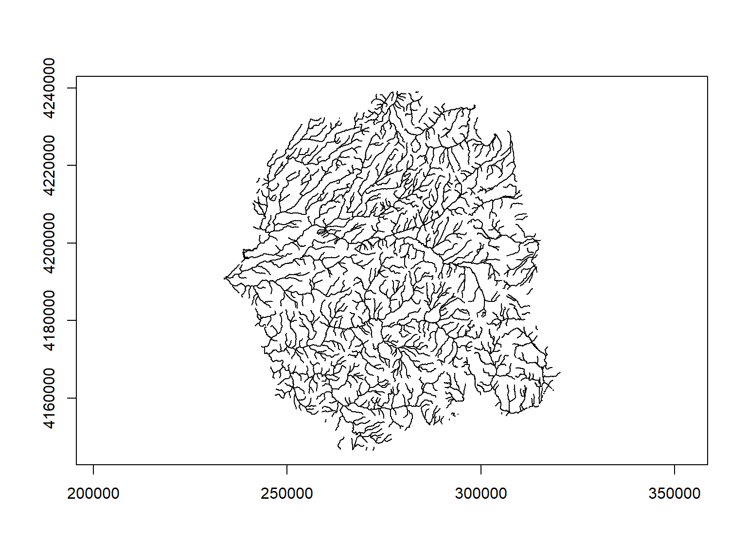
Step 4. Convert the ArcGIS Data Frame into a `sf` object

You can use arc.data2sf() to convert the ArcGIS data frame to sf:

yose_rivers_sf <- arc.data2sf(yose_rivers_adf)
class(yose_rivers_sf)

## [1] "sf"         "data.frame"

Plot to see how it looks:

plot(yose_rivers_sf %>% st_geometry(), axes=TRUE)

Writing to geodatabases

Write sf objects to a geodatabase with:

arc.write(path, data, overwrite)

Importing Data from ArcGIS.com

Option 1: Import the JSON

If the feature service you’re interested in is:

public on ArcGIS.com (or an ArcGIS Entrprise Server), and
was published with JSON enabled

…then you can import it directly (without arcgisbinding).

The first step is to look for a link to get the JSON (example):

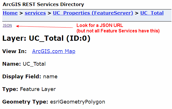
Not all feature services have a JSON link. It depends on whether JSON sharing was enabled by person who published the layer.

If it doesn’t have a JSON link, you can still import the layer into R using the R-ArcGIS Bridge (see below).

Normally you can import GeoJSON files with st_read(). Let’s try:

library(sf)
library(dplyr)

uc_props_url <- "https://services2.arcgis.com/wx8u046p68e0iGuj/arcgis/rest/services/UC_Properties/FeatureServer/0?f=pjson"

try(uc_props_sf <- st_read(uc_props_url))

## Warning in CPL_read_ogr(dsn, layer, query, as.character(options), quiet, : GDAL Error 1: Invalid FeatureCollection
## object. Missing 'features' member.

## Warning in CPL_read_ogr(dsn, layer, query, as.character(options), quiet, : GDAL Error 4: Failed to read ESRIJSON data

## Error : Cannot open "https://services2.arcgis.com/wx8u046p68e0iGuj/arcgis/rest/services/UC_Properties/FeatureServer/0?f=pjson"; The file doesn't seem to exist.

OH NO - ERROR!!

ESRI JSON is not standard GeoJSON!

`esri2sf` to the rescue!

Fortunately there’s a package for that! Thanks to Yongha Hwang, who wrote esri2sf to help people import ESRI JSON into R as sf data frames.

To use esri2sf, you simply enter the URL to the Feature Class (excluding any parameters in the URL) to esri2sf():

## If you don't have it esri2sf installed, you can install it with:
## remotes::install_github("yonghah/esri2sf")

library(esri2sf)

## Note the URL you pass to esri2sf should not include anything after /0
uc_props_url <- "https://services2.arcgis.com/wx8u046p68e0iGuj/arcgis/rest/services/UC_Properties/FeatureServer/0"

uc_props_sf <- esri2sf(uc_props_url)

## [1] "Feature Layer"
## [1] "esriGeometryPolygon"
## [1] "Coordinate Reference System: 3857"

uc_props_sf

## Simple feature collection with 102 features and 6 fields
## Geometry type: MULTIPOLYGON
## Dimension:     XY
## Bounding box:  xmin: -123.7662 ymin: 32.75285 xmax: -114.8905 ymax: 41.96819
## Geodetic CRS:  WGS 84
## First 10 features:
##    OBJECTID            name Campus          Type Shape__Area Shape__Length                          geoms
## 1         1 Sierra Foothill UC ANR Field Station 38372942.07    51745.3835 MULTIPOLYGON (((-121.3015 3...
## 2         2     South Coast UC ANR Field Station  1169888.33     4357.4984 MULTIPOLYGON (((-117.7136 3...
## 3         3          Hansen UC ANR Field Station   158425.23     1653.1777 MULTIPOLYGON (((-119.1049 3...
## 4         4         Kearney UC ANR Field Station  2058980.90     8801.7717 MULTIPOLYGON (((-119.5026 3...
## 5         5        Lindcove UC ANR Field Station  1075053.61     4553.3554 MULTIPOLYGON (((-119.0623 3...
## 6         6        Lindcove UC ANR Field Station    27609.79      666.4457 MULTIPOLYGON (((-119.054 36...
## 7         7   Intermountain UC ANR Field Station  1056001.61     5200.2187 MULTIPOLYGON (((-121.467 41...
## 8         8          Desert UC ANR Field Station  1456537.02     6297.5787 MULTIPOLYGON (((-115.4389 3...
## 9         9        Westside UC ANR Field Station  1963226.98     5960.1049 MULTIPOLYGON (((-120.1215 3...
## 10       10         Hopland UC ANR Field Station 35502119.75    32375.9906 MULTIPOLYGON (((-123.1032 3...

Plot to make sure:

library(tmap)
tmap_mode("view")

## tmap mode set to interactive viewing

tm_shape(uc_props_sf %>% select(name, Campus, Type)) +
  tm_polygons("Type")

Importing Data from ArcGIS.com

Option 2: Use the R-ArcGIS Bridge

Whether or not a feature service allows JSON downloading, you can import it into R using the R-ArcGIS Bridge.

The first step is to feed the reference URL into arc.open():

uc_props_url <- "https://services2.arcgis.com/wx8u046p68e0iGuj/arcgis/rest/services/UC_Properties/FeatureServer/0"

## Create a connect to the 'Rivers' feature class
uc_props_ftsrv_con <- arc.open(path = uc_props_url)

## Display info (metadata)
uc_props_ftsrv_con

## dataset_type    : FeatureClass
## path            : https://services2.arcgis.com/wx8u046p68e0iGuj/arcgis/rest/services/UC_Properties/FeatureServer/0 
## fields          : OBJECTID, name, Campus, Type, Shape__Area, Shape__Length, Shape
## extent          : xmin=-13777593, ymin=3862545, xmax=-12789550, ymax=5156216
## geometry type   : Polygon, has ZM
## WKT             : PROJCS["WGS_1984_Web_Mercator_Auxiliary_Sphere",GEOGCS["GCS_...
## WKID            : 3857

From there you would use arc.select() as usual to import the file into R, followed by arc.data2sf() to convert it to a sf data frame:

uc_props_ftsrv_sf <- arc.select(uc_props_ftsrv_con) %>% 
  arc.data2sf()

uc_props_ftsrv_sf

## Simple feature collection with 102 features and 6 fields
## Geometry type: GEOMETRY
## Dimension:     XYZM
## Bounding box:  xmin: -13777590 ymin: 3862545 xmax: -12789550 ymax: 5156216
## z_range:       zmin: 0 zmax: 0
## m_range:       mmin: 0 mmax: 0
## Projected CRS: WGS 84 / Pseudo-Mercator
## First 10 features:
##    OBJECTID            name Campus          Type Shape__Area Shape__Length                           geom
## 1         1 Sierra Foothill UC ANR Field Station 38372942.07    51745.3835 POLYGON ZM ((-13503217 4764...
## 2         2     South Coast UC ANR Field Station  1169888.33     4357.4984 POLYGON ZM ((-13103815 3987...
## 3         3          Hansen UC ANR Field Station   158425.23     1653.1777 POLYGON ZM ((-13258701 4072...
## 4         4         Kearney UC ANR Field Station  2058980.90     8801.7717 MULTIPOLYGON ZM (((-1330296...
## 5         5        Lindcove UC ANR Field Station  1075053.61     4553.3554 POLYGON ZM ((-13253954 4350...
## 6         6        Lindcove UC ANR Field Station    27609.79      666.4457 POLYGON ZM ((-13253031 4350...
## 7         7   Intermountain UC ANR Field Station  1056001.61     5200.2187 POLYGON ZM ((-13521647 5155...
## 8         8          Desert UC ANR Field Station  1456537.02     6297.5787 POLYGON ZM ((-12850595 3870...
## 9         9        Westside UC ANR Field Station  1963226.98     5960.1049 POLYGON ZM ((-13371864 4347...
## 10       10         Hopland UC ANR Field Station 35502119.75    32375.9906 POLYGON ZM ((-13703787 4727...

Importing Data from an ArcGIS Data Portal

You can also import protected data from AGOL. To verify you have access, make sure you’re signed-in to the portal you want to access in ArcGIS Pro. Then check the status of your portal connection in R:

arc.check_portal()

## *** Current
##   url        : https://www.arcgis.com/
##   version    : NA
##   user       : andlyons_UCANR
##   organization   : UC Agriculture and Natural Resources

If you need to import data from multiple portals, you can connect to additional portals using arc.portal_connect().

Once you’re logged into your portal, you can import feature classes as before with arc.open() followed by arc.select().

Example: Download a layer from Living Atlas

Living Atlas is a spatial data portal curated by ESRI. Accessing Living Portal requires an ArcGIS.com account. In this example we import a Living Atlas layer containing the locations of post offices in Hong Kong.

Step 1 is to find the URL for the feature service:

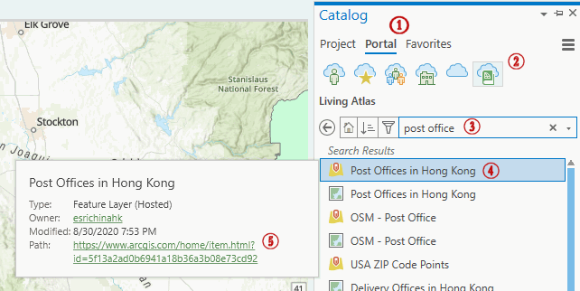
Once you have the URL to the feature class, you can import the data:

## Get the URL for the Feature Service
## NOTE: the URL should end with the name of a feature class, which could be a number
hk_postoffices_url <- "https://services3.arcgis.com/6j1KwZfY2fZrfNMR/arcgis/rest/services/Post_Offices_in_Hong_Kong/FeatureServer/0"

## Create the connection
hk_postoffices_con <- arc.open(path = hk_postoffices_url)
class(hk_postoffices_con)

## [1] "arc.feature_impl"
## attr(,"package")
## [1] "arcgisbinding"

hk_postoffices_con

## dataset_type    : FeatureClass
## path            : https://services3.arcgis.com/6j1KwZfY2fZrfNMR/arcgis/rest/services/Post_Offices_in_Hong_Kong/FeatureServer/0 
## fields          : OBJECTID, OBJECTID_1, GMID, Dataset, Facility_Name, Address, <U+6578><U+64DA><U+96C6>, 
## fields          : <U+8A2D><U+65BD><U+540D><U+7A31>, <U+5730><U+5740>, District, <U+5730><U+5340>, Opening_Hours, 
## fields          : <U+958B><U+653E><U+6642><U+9593>, Telephone, <U+806F><U+7D61><U+96FB><U+8A71>, Fax_Number, 
## fields          : <U+50B3><U+771F><U+865F><U+78BC>, Email_Address, <U+96FB><U+90F5><U+5730><U+5740>, Website, 
## fields          : <U+7DB2><U+9801>, Scope_of_Services, <U+670D><U+52D9><U+7BC4><U+570D>, Remarks, <U+5099><U+8A3B>, 
## fields          : Northing, Easting, Latitude, Longitude, Last_Update, Shape
## extent          : xmin=12674870, ymin=2536375, xmax=12720737, ymax=2577170
## geometry type   : Point, has Z
## WKT             : PROJCS["WGS_1984_Web_Mercator_Auxiliary_Sphere",GEOGCS["GCS_...
## WKID            : 3857

## Import the data and convert to sf
hk_postoffices_sf <- hk_postoffices_con %>% 
  arc.select() %>% 
  arc.data2sf() %>% 
  select(Facility_Name, Address, District)

## Plot it to make sure it worked
tmap_mode("view")

## tmap mode set to interactive viewing

tm_shape(hk_postoffices_sf) + 
  tm_symbols(size = 0.5)

The URL passed to arc.open() should end with the name of a feature class (which may just be a number):

https://services3.arcgis.com/…/rest/services/Post_Offices/FeatureServer/0

Importing with an Attribute Filter

Quite often a GIS layer you’re trying to import includes a lot more features than you actually need. Rather than import all them and filter out the ones you need, arc.select() let’s you pass a filter expression that the server will use to filter features based on their attribute values, and only send you the features that meet the expression.

Example: Import California Zip Code Center Points from Living Atlas

There are over 41,000 zip codes in the USA, but only 2500 in California. In this example we’ll import the zip code center points for California using an attribute filter.

First create a connection to the Feature Service:

## Get the URL for the Feature Service
usa_zip_pts_url <- "https://services.arcgis.com/P3ePLMYs2RVChkJx/arcgis/rest/services/USA_ZIP_Code_Points_analysis/FeatureServer/0"

## Create the connection
usa_zip_pts_con <- arc.open(path = usa_zip_pts_url)

## View the metadata
usa_zip_pts_con

## dataset_type    : FeatureClass
## path            : https://services.arcgis.com/P3ePLMYs2RVChkJx/arcgis/rest/services/USA_ZIP_Code_Points_analysis/FeatureServer/0 
## fields          : OBJECTID, ZIP_CODE, PO_NAME, STATE, ZIP_TYPE, POPULATION, SQMI, Shape
## extent          : xmin=-19676856, ymin=1490010, xmax=16126807, ymax=11314590
## geometry type   : Point
## WKT             : PROJCS["WGS_1984_Web_Mercator_Auxiliary_Sphere",GEOGCS["GCS_...
## WKID            : 3857

Next we can import the features with arc.select(), adding a simple expression for the where_clause argument:

ca_zip_pts_sf <- usa_zip_pts_con %>% 
  arc.select(where_clause = "STATE = 'CA'") %>% 
  arc.data2sf() %>% 
  select(ZIP_CODE, PO_NAME, STATE, ZIP_TYPE)

tm_shape(ca_zip_pts_sf) +
  tm_dots()

To download data from an ArcGIS server with a spatial filter, see arcpullr.

Sharing Spatial Data via AGOL

If you want to share your spatial data on ArcGIS.com or an ArcGIS Enterprise Server (e.g., in a web map), you have to save it as a GIS file that you can then upload to AGOL.

But not all GIS file formats are created equal! Some can be added to a web map on AGOL, some not. Some can be published as a hosted web layer, some not. The functionality you can get in AGOL for each file format is summarized below (Details):

AGOL Functionality	GeoJSON	Shapefile	KML	GeoPackage	Geodatabase
Display in a web map	✔	✔	✔
Publish as a hosted web layer	✔	✔			✔
Download	✔	✔	✔	✔	✔

When in doubt, upload a GeoJSON file. It has all the functionality on AGOL, and doesn’t have the limitations on attribute tables that KML and Shapefiles have.

ArcGIS Pro provides additional options when it comes to publishing data on AGOL. For this approach, export your data from R to a geodatabase, then connect to the geodatabase in ArcGIS Pro.

Summary

Today we saw how to:

import data from a geodatabase using the R-ArcGIS bridge
two ways to import online data from ArcGIS.com and ArcGIS Enterprise servers:

esri2sf if the data are public and shared as JSON
R-ArcGIS Bridge for all other situations

Tutorials and Exercises from ESRI:

Spatial Data Analysis with R Society for Conservation GIS, July 2021

Cross-Walking R and ArcGIS Pro

R-ArcGIS Bridge

Installation

What You Can Do with the R-ArcGIS Bridge

Example: Import data from a Geodatabase

Step 1. Load arcgisbinding and verify the license

Step 2. Create a ‘Connection Object’ to a feature class in a geodatabase

Step 3. Import the Feature Class into R as an “ArcGIS data frame”

Step 4. Convert the ArcGIS Data Frame into a sf object

Writing to geodatabases

Importing Data from ArcGIS.com

Option 1: Import the JSON

esri2sf to the rescue!

Importing Data from ArcGIS.com

Option 2: Use the R-ArcGIS Bridge

Importing Data from an ArcGIS Data Portal

Example: Download a layer from Living Atlas

Importing with an Attribute Filter

Example: Import California Zip Code Center Points from Living Atlas

Sharing Spatial Data via AGOL

Summary

Spatial Data Analysis with R
Society for Conservation GIS, July 2021

Step 1. Load `arcgisbinding` and verify the license

Step 4. Convert the ArcGIS Data Frame into a `sf` object

`esri2sf` to the rescue!