Spatial Data Analysis with R
Society for Conservation GIS, July 2021

Common Manipulations for sf Objects

Simple Features

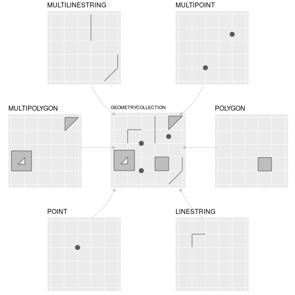
simple features is an ISO standard for storing and accessing spatial data. It is widely adopted in spatial databases, open source formats like GeoJSON, GIS software, tools, etc.

sf employs a standard called “Well Known Text” (WKT) to encode the geometry. WKT is a very simple written representation of the ‘connect-the-dots’ vector data model.

Geometry Sample WKT
point POINT (2 4)
multipoint MULTIPOINT (2 2, 3 3, 3 2)
linestring LINESTRING (0 3, 1 4, 2 3)
polygon POLYGON ((1 0, 3 4, 5 1, 1 0))

Import the Yosemite points-of-interest Shapefile.

library(sf)

## Import the Yosemite Points-of-Interest Shapefile
yose_poi_utm <- st_read(dsn="./data", layer="yose_poi")

## View column names in the attribute table
names(yose_poi_utm)

## Plot the points
plot(yose_poi_utm %>% st_geometry(), pch=16, asp=1, cex=0.5, axes=TRUE)
## Reading layer `yose_poi' from data source `D:\Workshops\R-Spatial\rspatial_mod\outputs\rspatial_data\data' using driver `ESRI Shapefile'
## Simple feature collection with 2720 features and 30 fields
## Geometry type: POINT
## Dimension:     XY
## Bounding box:  xmin: 246416.2 ymin: 4153717 xmax: 301510.7 ymax: 4208419
## Projected CRS: NAD83 / UTM zone 11N
##  [1] "OBJECTID"   "POINAME"    "POIALTNAME" "POILABEL"   "POIFEATTYP" "POITYPE"    "UNITCODE"  
##  [8] "UNITNAME"   "GROUPCODE"  "REGIONCODE" "ISEXTANT"   "MAPMETHOD"  "MAPSOURCE"  "SRCESCALE" 
## [15] "SOURCEDATE" "XYERROR"    "LOCATIONID" "ASSETID"    "NOTES"      "DISTRIBUTE" "RESTRICTIO"
## [22] "CREATEDATE" "CREATEUSER" "EDITDATE"   "EDITUSER"   "FEATUREID"  "GEOMETRYID" "PLACESID"  
## [29] "GlobalID"   "TAGS"       "geometry"

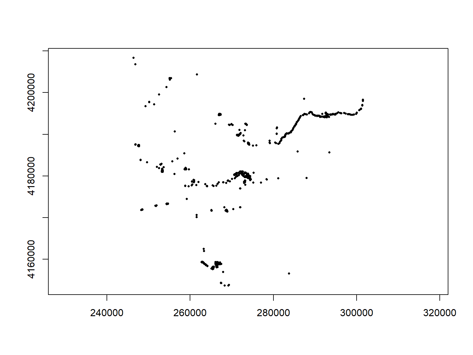
Take a closer look at the geometry column:

class(yose_poi_utm$geometry)
head(yose_poi_utm[, "geometry"])
## [1] "sfc_POINT" "sfc"      
## Simple feature collection with 6 features and 0 fields
## Geometry type: POINT
## Dimension:     XY
## Bounding box:  xmin: 260859.4 ymin: 4153717 xmax: 270931.1 ymax: 4179771
## Projected CRS: NAD83 / UTM zone 11N
##                   geometry
## 1 POINT (260859.4 4178493)
## 2 POINT (264115.4 4158415)
## 3 POINT (268276.8 4153717)
## 4 POINT (268620.1 4178344)
## 5 POINT (269052.6 4178870)
## 6 POINT (270931.1 4179771)

The geometry column of a sf object does not have to be called ‘geometry’. You can view the column name by running attr(x, "sf_column") where x is a sf object.

The features in a sf object can be a mix of points, lines, and polyons. The data class of the geometry column is therefore sfc (simple features collection).

Other properties of sf objects

Bounding box

It’s often useful to view the metadata of a sf object. You can get the bounding box (aka extent) with st_bbox().

st_bbox(yose_poi_utm)
##      xmin      ymin      xmax      ymax 
##  246416.2 4153717.3  301510.7 4208419.0

Coordinates

To extract the coordinates of a sf object as a matrix, use st_coordinates().

x <- st_coordinates(yose_poi_utm)
head(x)
##          X       Y
## 1 260859.4 4178493
## 2 264115.4 4158415
## 3 268276.8 4153717
## 4 268620.1 4178344
## 5 269052.6 4178870
## 6 270931.1 4179771

Projections

Projections are particularly important whenever you want to:

The more generic term for projections as is Coordinate Reference System (CRS).

CRS also includes unprojected geographic coordinates (longitude & latitude).

A CRS has three parts:

  1. a mathematical representation of the Earth (datum)
  2. a 2D to 3D transformation model (projected CRS’s)
  3. an origin

CRS functions

All sf objects are able to store projection info.

st_read() imports the CRS info from standard GIS file formats

st_crs() creates, views, or assigns the CRS

st_transform() (re)projects sf objects into a different crs

Using Established CRSs

The sf package uses the PROJ.4 library for established CRS. It provides two ways to specify a known projection:

EPSG codes were developed by the European Petroluem Survey Group.

The following are equivalent:

st_crs("+init=epsg:3857")
st_crs(3857)

If you happen to know the proj4string, you can use it also

st_crs("+proj=utm +zone=10 +ellps=GRS80 +datum=NAD83 +units=m +no_defs")
## Coordinate Reference System:
##   User input: +proj=utm +zone=10 +ellps=GRS80 +datum=NAD83 +units=m +no_defs 
##   wkt:
## PROJCRS["unknown",
##     BASEGEOGCRS["unknown",
##         DATUM["North American Datum 1983",
##             ELLIPSOID["GRS 1980",6378137,298.257222101,
##                 LENGTHUNIT["metre",1]],
##             ID["EPSG",6269]],
##         PRIMEM["Greenwich",0,
##             ANGLEUNIT["degree",0.0174532925199433],
##             ID["EPSG",8901]]],
##     CONVERSION["UTM zone 10N",
##         METHOD["Transverse Mercator",
##             ID["EPSG",9807]],
##         PARAMETER["Latitude of natural origin",0,
##             ANGLEUNIT["degree",0.0174532925199433],
##             ID["EPSG",8801]],
##         PARAMETER["Longitude of natural origin",-123,
##             ANGLEUNIT["degree",0.0174532925199433],
##             ID["EPSG",8802]],
##         PARAMETER["Scale factor at natural origin",0.9996,
##             SCALEUNIT["unity",1],
##             ID["EPSG",8805]],
##         PARAMETER["False easting",500000,
##             LENGTHUNIT["metre",1],
##             ID["EPSG",8806]],
##         PARAMETER["False northing",0,
##             LENGTHUNIT["metre",1],
##             ID["EPSG",8807]],
##         ID["EPSG",16010]],
##     CS[Cartesian,2],
##         AXIS["(E)",east,
##             ORDER[1],
##             LENGTHUNIT["metre",1,
##                 ID["EPSG",9001]]],
##         AXIS["(N)",north,
##             ORDER[2],
##             LENGTHUNIT["metre",1,
##                 ID["EPSG",9001]]]]

Common EPSG Numbers

Geographic CRSs

4326. Geographic, WGS84 (default for lon/lat)
4269. Geographic, NAD83 (USA Fed agencies like Census)

Projected CRSs

5070. USA Contiguous Albers Equal Area Conic
3310. CA ALbers Equal Area
32610. UTM Zone 10, WGS84 (Northern Cal)
32611. UTM Zone 11, WGS84 (Southern Cal)
3857. Web Mercator (web maps)

The one-stop shop for finding proj4 strings and epsg numbers is http://www.spatialreference.org. (Google usually works also).

Reference code for your convenience:

## Some common epsg numbers in California
epsg_geo_wgs84 <- 4326
epsg_geo_nad83 <- 4269
epsg_utm10n_wgs84 <- 32610
epsg_utm11n_wgs84 <- 32611
epsg_utm10n_nad83 <- 26910
epsg_utm11n_nad83 <- 26911
epsg_webmerc <- 3857
epsg_caalbers <- 3310

To view all EPSG codes (>5,500), run rgdal::make_EPSG()

See also Projection and Datum Guidelines for California (CDFW)

View or Assign the CRS

View the CRS

st_crs(yose_trails)
## Coordinate Reference System:
##   User input: NAD83 / UTM zone 11N 
##   wkt:
## PROJCRS["NAD83 / UTM zone 11N",
##     BASEGEOGCRS["NAD83",
##         DATUM["North American Datum 1983",
##             ELLIPSOID["GRS 1980",6378137,298.257222101,
##                 LENGTHUNIT["metre",1]]],
##         PRIMEM["Greenwich",0,
##             ANGLEUNIT["degree",0.0174532925199433]],
##         ID["EPSG",4269]],
##     CONVERSION["UTM zone 11N",
##         METHOD["Transverse Mercator",
##             ID["EPSG",9807]],
##         PARAMETER["Latitude of natural origin",0,
##             ANGLEUNIT["degree",0.0174532925199433],
##             ID["EPSG",8801]],
##         PARAMETER["Longitude of natural origin",-117,
##             ANGLEUNIT["degree",0.0174532925199433],
##             ID["EPSG",8802]],
##         PARAMETER["Scale factor at natural origin",0.9996,
##             SCALEUNIT["unity",1],
##             ID["EPSG",8805]],
##         PARAMETER["False easting",500000,
##             LENGTHUNIT["metre",1],
##             ID["EPSG",8806]],
##         PARAMETER["False northing",0,
##             LENGTHUNIT["metre",1],
##             ID["EPSG",8807]]],
##     CS[Cartesian,2],
##         AXIS["(E)",east,
##             ORDER[1],
##             LENGTHUNIT["metre",1]],
##         AXIS["(N)",north,
##             ORDER[2],
##             LENGTHUNIT["metre",1]],
##     USAGE[
##         SCOPE["unknown"],
##         AREA["North America - 120°W to 114°W and NAD83 by country"],
##         BBOX[30.88,-120,83.5,-114]],
##     ID["EPSG",26911]]

Set the CRS

Occasionally, you have a sf object that doesn’t have a CRS recorded. This is most common when you are importing a CSV file and are turning it into a sf object. In thse cases, you can use st_crs() to assign the CRS.

st_crs(my_gps_pts) <- 4326

Note: this is not the same as projecting data. You’re simply telling it the CRS.

Projecting Data

You can project data from one CRS to another with:

st_transform(sf_object, new_crs)

Let’s ‘unproject’ the Yosemite trails layer from UTM to geographic coordinates.

## (Un)project the trails layer to geographic coordinates
yose_trails_ll <- st_transform(yose_trails, 4269)

Now that the trails are in geographic coordinates, we can overlay them on the boundary and historical points.

## Plot the trails, then overlay the historic points and park boundary
plot(yose_trails_ll %>% st_geometry(), asp=1, col="bisque3", axes=T, main="Yosemite National Park")
plot(yose_hp %>% st_geometry(), col="gray30", pch=16, add=TRUE)
plot(yose_bnd_ll %>% st_geometry(), col=NA, border="chartreuse4", lwd=3, add=TRUE)

You can project one layer to match another without knowing the exact CRS. Just extract the CRS of the layer you’re trying to match with st_crs(), and use that as the second argument in st_transform().

yose_trails_ll <- st_transform(yose_trails, st_crs(yose_bnd_ll))

Import the Yosemite roads and add those to your map. You may use the code below to get started.

## Get the path to the geodatabase 
gdbroads_fn <- "./data/yose_roads.gdb"
file.exists(gdbroads_fn)

## Import the roads layer
yose_roads_utm <- st_read(gdbroads_fn, layer="Yosemite_Roads")

[Solution]

## (Un)project the roads layer to geographic coordinates
yose_roads_ll <- st_transform(yose_roads_utm, 4269)

## Plot all four layers
plot(yose_trails_ll %>% st_geometry(), asp=1, col="bisque3", axes=T, main="Yosemite")
plot(yose_roads_ll %>% st_geometry(), col="navyblue", lwd=1, lty=5, add=TRUE)
plot(yose_hp %>% st_geometry(), col="gray30", pch=16, add=TRUE)
plot(yose_bnd_ll %>% st_geometry(), col=NA, border="chartreuse4", lwd=3, add=TRUE)
## [1] TRUE

Exporting sf objects to disk

You can export sf objects as Shapefiles and other formats using st_write()

If you name the output file with a standard extension (e.g., .shp, .kml), st_write() will know which format to use. Otherwise you have to add the driver argument.

## For testing purposes, pull out fires from the 2000s
yose_fires20_pt <- yose_fires_pt %>% filter(DECADE == 2000)

## Export to Shapefile
st_write(yose_fires20_pt, 
         dsn="~yose_fires20s_pt.shp")

## Export to GeoPackage
st_write(yose_fires20_pt, 
         dsn="~yose_fires.gpkg", 
         layer="yose_fires20s")

By default, st_write() will throw an error if the output file already exists. To overwrite existing data (not recommended), add delete_dsn = TRUE.

Converting sf ↔︎ sp

If you need to convert a sf object to a sp object (for backwards compatibility, for example), use as(x, "Spatial"):

Example:

## Convert sf to sp
yose_fires_sp <- as(yose_fires_pt, "Spatial")
class(yose_fires_sp)

See also:

Summary

Today we saw how to:

Additional Resources


Next: Tables 101