Building a Map with `tmap`

A tmap object (aka tmap-element) is constructed by connecting a series of functions that:

set the data source for each layer
draw features on the map
add elements such as scale bar and north arrows
customize the layout, including title, legend placement, etc.

Example of a complete map definition:

tm_shape(yose_bnd_ll) +                             ## Define first layer data source
  tm_polygons() +                                   ## Add features from the source 
tm_shape(yose_hp_ll) +                              ## Add another source (layer)
  tm_symbols(size=0.5, col="navy") +                ## Throw on point symbols
tm_shape(yose_roads_utm) +                          ## Add still another source (layer)
  tm_lines(col="gray60", lwd=1.5, lty="dotted") +   ## Add lines
tm_scale_bar(position=c("right", "bottom")) +       ## Global element - scale bar
tm_compass(position=c("left", "bottom")) +          ## Global element - north arrow
tm_style("cobalt")                                  ## Global style preset (default colors)

tmap functions are joined with + rather than %>%

breaking a tmap expression across lines and using indents can improve readability

tmap layers

1) Each layer starts with tm_shape(), which specifies the data source, projection, and bounding box.

2) You then add features to the map with one of the following drawing functions that start with tm_...()

Feature Class	Drawing Function(s)
points	tm_symbols(), tm_dots()
lines	tm_lines()
polygons	tm_polygons(), tm_fill(), tm_borders()
rasters	tm_raster(), tm_rgb()
labels	tm_text()

Functions that draw features on the map are also known as aesthetics.

Example: A One-Layer Map

library(tmap)
yose_bnd_ll <- st_read(dsn="./data", layer="yose_boundary")

## Reading layer `yose_boundary' from data source `D:\Workshops\R-Spatial\rspatial_mod\outputs\rspatial_data\data' using driver `ESRI Shapefile'
## Simple feature collection with 1 feature and 11 fields
## Geometry type: POLYGON
## Dimension:     XY
## Bounding box:  xmin: -119.8864 ymin: 37.4947 xmax: -119.1964 ymax: 38.18515
## Geodetic CRS:  North_American_Datum_1983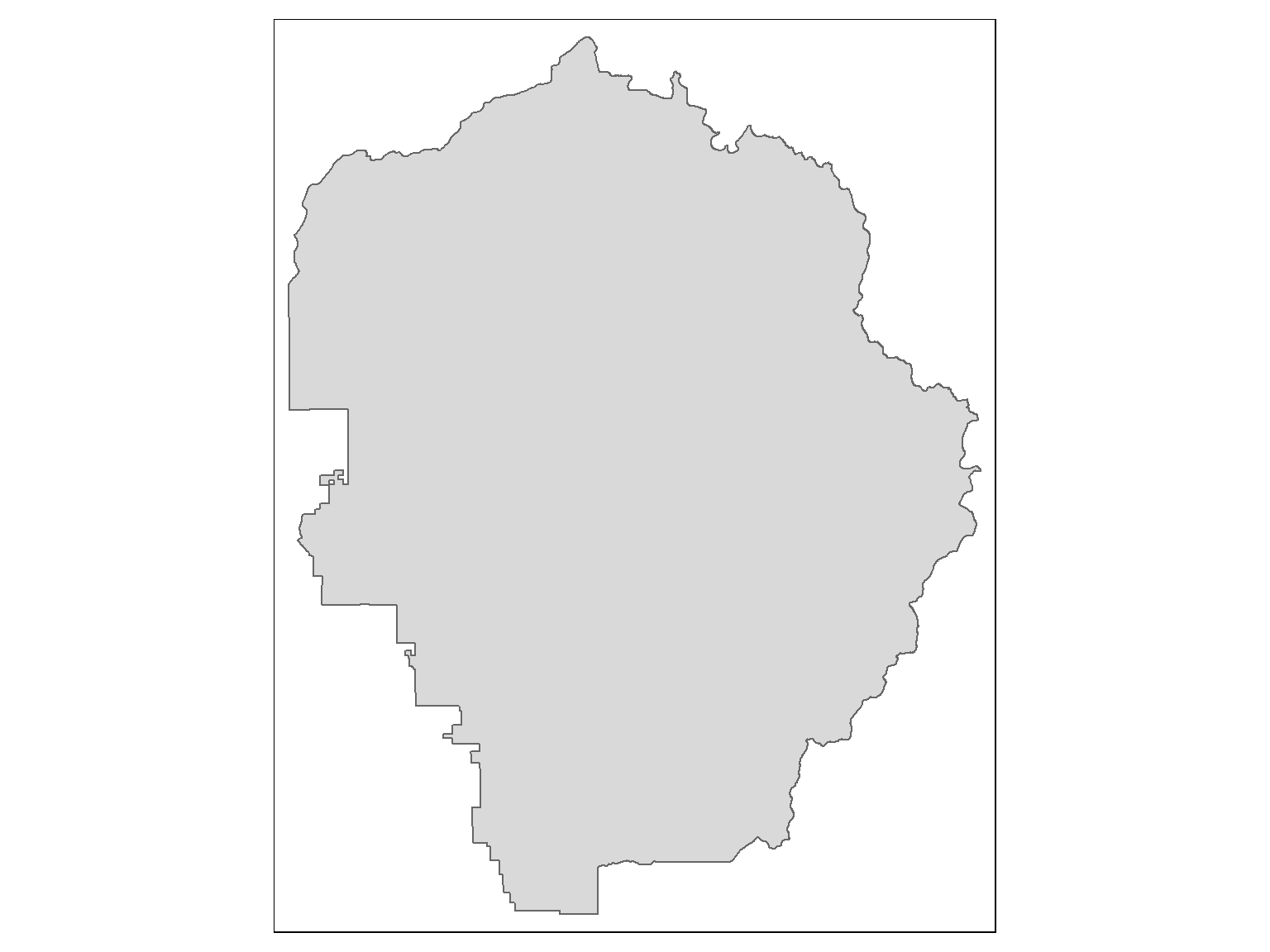

tm_shape(yose_bnd_ll) + tm_polygons()

Multi-layered maps

To add additional layers you simply add more tm_shape() and tm_xxx() functions.

Add the historic points to our map:

yose_hp_ll <- st_read("./data/yose_historic_pts.kml", layer="yose_historic_places", quiet = TRUE)

## Add a second layer
tm_shape(yose_bnd_ll) + 
  tm_polygons() + 
tm_shape(yose_hp_ll) + 
  tm_symbols()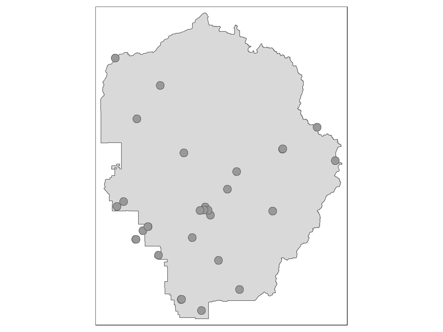

Reprojection on the Fly

tmap will automatically reproject layers to match the first one (if needed).

Example

Projection on-the-fly allows us to overlay the roads layer (in UTM) on the park boundary (in geographic coordinates).

Import the roads:

yose_roads_utm <- st_read("./data/yose_roads.gdb", layer="Yosemite_Roads", quiet = TRUE)
st_crs(yose_roads_utm)$proj4string

## [1] "+proj=utm +zone=11 +datum=NAD83 +units=m +no_defs"

The roads are in UTM, while the other layers are in geographic coordinates. Add them anyway!

tm_shape(yose_bnd_ll) + 
  tm_polygons() + 
tm_shape(yose_hp_ll) + 
  tm_symbols() +
tm_shape(yose_roads_utm) +
  tm_lines()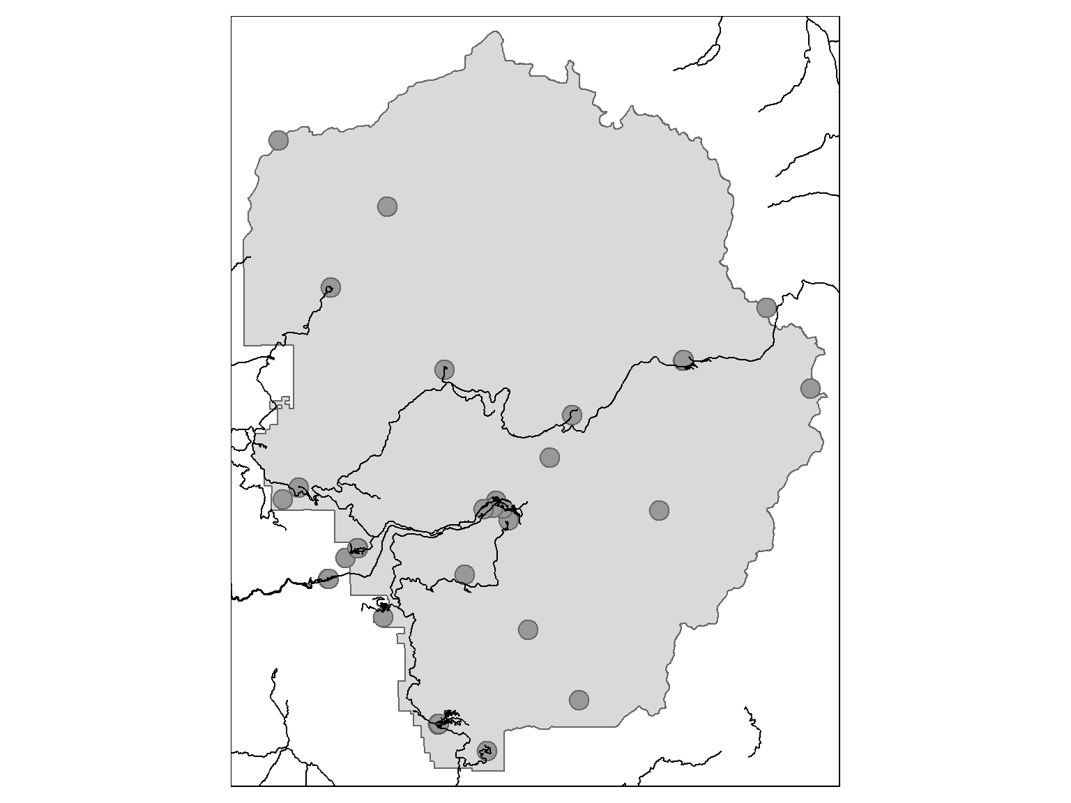

Just because tmap can reproject on the fly, doesn’t mean its a good idea.

Projecting all your data into the same CRS when you import is generally preferred - projection only needs to be done once.

Symbology

There are many arguments you can use to customize the symbology of layers. Example:

tm_shape(yose_bnd_ll) + 
  tm_polygons(col = "ivory") + 
tm_shape(yose_hp_ll) + 
  tm_symbols(size=0.5, col="forestgreen") +
tm_shape(yose_roads_utm) +
  tm_lines(col="gray60", lwd=1.5, lty="dotted")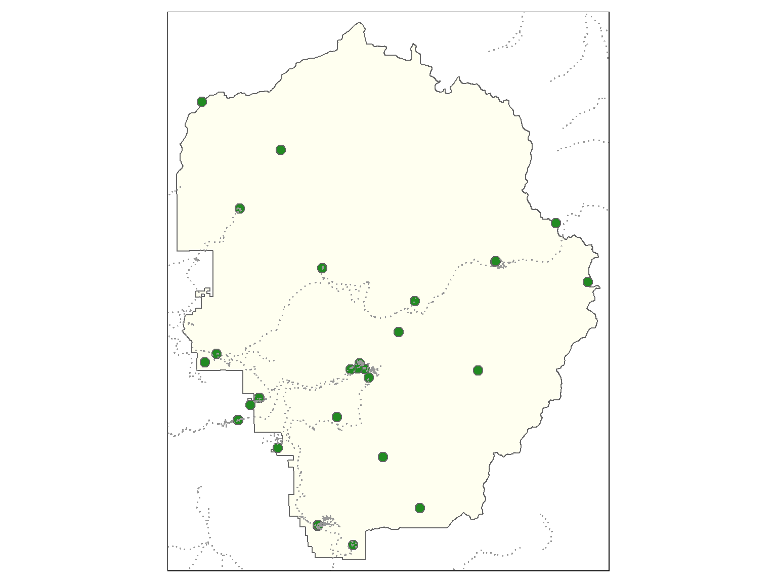

Read the help pages for each drawing function to see which arguments are supported

Some of the more common symbology arguments include:

shape

size

scale

col

alpha

colorNA

border.col

border.lwd

border.alpha

lty

lwd

tmap has ‘presets’ of default symbology options. See tmap_style().

Symbolizing by Attribute Value

To symbolize features by an attribute value:

pass a column name as the col (color) argument in a drawing function
pass additional arguments in the drawing function to specify how the attribute values should be mapped to colors, (e.g., palette, number of beaks, etc.)

Example: Use a different color for each road type

The road type is saved in column YOSE_Type, so we pass that as the ‘color’ in tm_lines():

## Symbolize roads by type
tm_shape(yose_bnd_ll) + 
  tm_polygons(col = "gray95") + 
tm_shape(yose_hp_ll) + 
  tm_symbols(size = 0.5, col = "forestgreen") +
tm_shape(yose_roads_utm) +
  tm_lines(col = "YOSE_Type")

Tweaking the Legend

Tweak the legend with additional options passed to tm_legend() or tm_layout().

## Symbolize roads by type
tm_shape(yose_bnd_ll) + 
  tm_polygons(col="gray95") + 
tm_shape(yose_hp_ll) + 
  tm_symbols(size=0.5, col="forestgreen") +
tm_shape(yose_roads_utm) +
  tm_lines("YOSE_Type", title.col = "Roads") +
tm_layout(legend.outside = TRUE, legend.bg.color="white", legend.frame=TRUE, legend.text.size=1)

## Some legend labels were too wide. These labels have been resized to 0.83. Increase legend.width (argument of tm_layout) to make the legend wider and therefore the labels larger.

Anatomy of a Choropleth Map in `tmap`

Choropleth maps display geographical areas using colors, shading, and patterns in relation to a numeric data variable.

Example Choropleth Map:

Arguments that define the choropleth generally go inside drawing functions that display the features (e.g., tm_symbols(), tm_polygons(), tm_fill(), tm_borders()).

Arguments commonly used to make choropleth maps include:

col - the column that has the values

palette - a vector of colors, or a named color palette (to see a list of named palettes, run run tmaptools::palette_explorer())

n - number of ‘bins’ to create

style - how the ‘bins’ should be constructed (details):

discrete options: “cat”, “fixed”, “sd”, “equal”, “pretty”, “quantile”, “kmeans”, “hclust”, “bclust”, “fisher”, “jenks”, and “log10_pretty”`
continuous options: “cont”, “order”, “log10”

breaks - specific break points (when style = 'fixed')

Example: Map Population by County

Let’s plot county population using a choropleth map. First import the county layers:

## Load the counties
epsg_caalbers <- 3310

ca_cnty_alb <- sf::st_read("./data/ca_counties.geojson", quiet = TRUE) %>% 
  sf::st_transform(epsg_caalbers)

## View the attribute table:
ca_cnty_alb %>% sf::st_drop_geometry() %>% dplyr::slice(1:5)

##   STATEFP COUNTYFP LSAD       ALAND    AWATER CountyFIPS            CountyNAME POP2010 POP2011 POP2012 POP2013 POP2014     SQMI
## 1      06      099   22  3870792979  51176484      06099     Stanislaus County  515283  518270  522134  526286  531997  1494.52
## 2      06      075   22   121451664 479139414      06075  San Francisco County  805825  816239  829691  841138  852469    46.89
## 3      06      005   22  1539947591  29470575      06005         Amador County   37860   37520   37072   36602   36742   594.58
## 4      06      071   22 51947497395 123929658      06071 San Bernardino County 2041689 2064663 2080651 2093306 2112619 20057.04
## 5      06      091   22  2468686345  23299112      06091         Sierra County    3221    3104    3076    3040    3003   953.17

Here we’ll construct a tmap object using the values in the numeric POP2104 column.

tm_shape(ca_cnty_alb) +
  tm_polygons (col = "POP2014",                   ## col: the column that contains the values
       n = 10,                                    ## n: number of bins
       style = "cont",                            ## style: method to create the bins
       palette = "YlOrRd",                        ## palette: a named palette or a vector of colors
       colorNA = "grey50",                        ## colorNA: the color to use for NA values
       legend.format = list(big.num.abbr = NA),   ## legend options  
       legend.reverse = FALSE ,                   ## legend.reverse: reverse the legend
       title = "2014 Population"                  ## title: title of the legend element
    ) + 
  tm_layout(legend.position = c("right", "top")) +
  tm_scale_bar(position = c("left", "bottom"))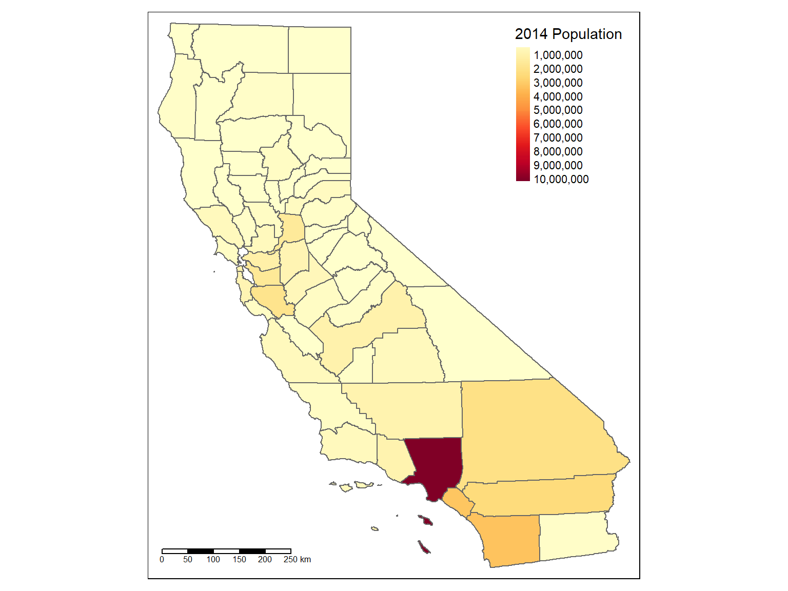

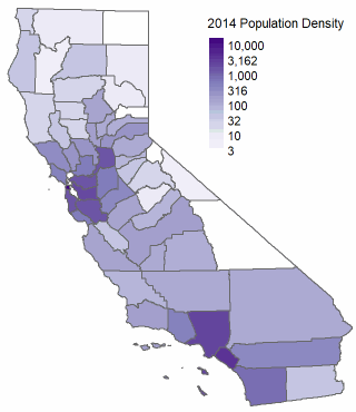
Make a map of the 2014 population density per county (i.e., population / square mile). Use a monochromatic color ramp (e.g., ‘Purples’). Hint

Create the column first using dplyr::mutate()

Because California’s population at the county level is so skewed (thanks LA!), consider using the ‘log10’ style to scale the values logarithmically.

Solution

## Compute the pouplation per square mile
ca_cnty_alb <- ca_cnty_alb %>% mutate(pop_density_2014 = POP2014 / SQMI)
summary(ca_cnty_alb$pop_density_2014)

## Create the map definition
mymap <- tm_shape(ca_cnty_alb) +
  tm_polygons (col = "pop_density_2014",                 ## col: the column that contains the values
               n = 10,                                   ## n: number of bins
               style = "log10",                          ## style: method to create the bins
               palette = "Purples",                      ## palette: a named palette or a vector of colors
               colorNA = "grey50",                       ## colorNA: the color to use for NA values
               legend.format = list(big.num.abbr = NA),  ## legend options  
               legend.reverse = TRUE ,                   ## legend.reverse: reverse the legend
               title = "2014 Population Density"         ## title: title of the legend element
  ) + 
  tm_layout(legend.position = c("right", "top")) +
  tm_scale_bar(position = c("left", "bottom"))

mymap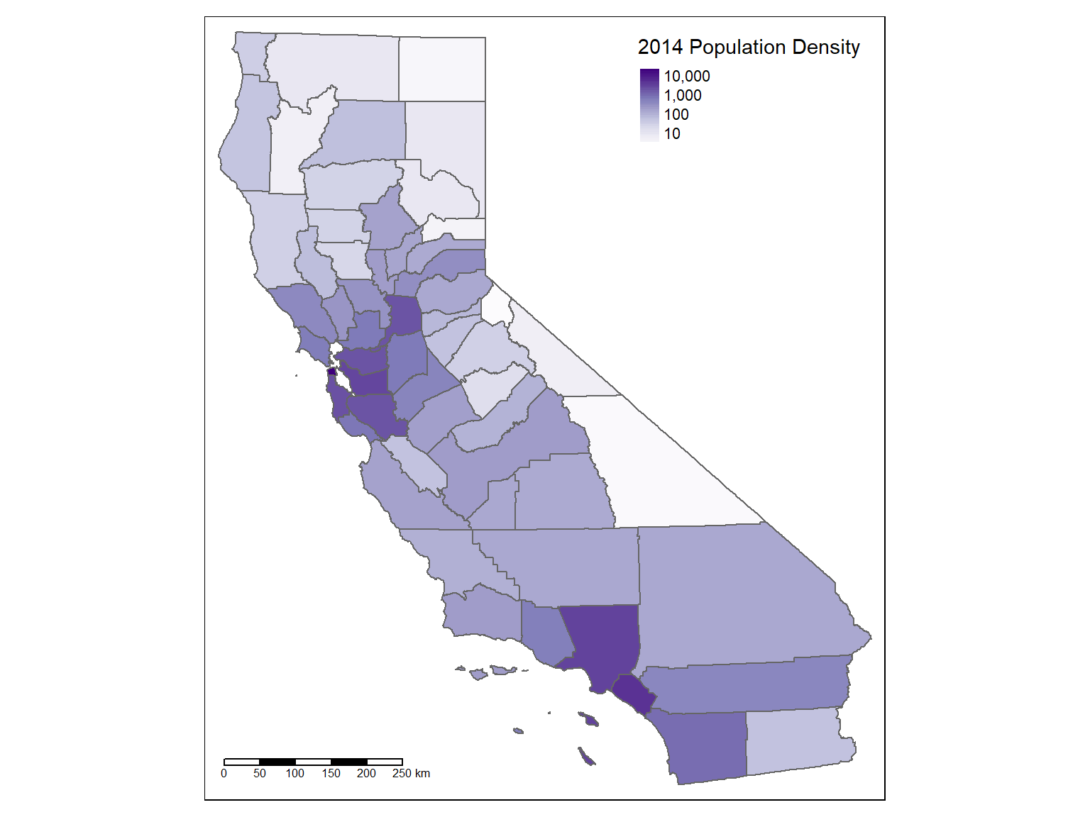

##      Min.   1st Qu.    Median      Mean   3rd Qu.      Max. 
##     1.512    25.555   107.375   696.709   347.779 18180.188

Raster Layers

You can draw a single-layer raster in your tmap object with tm_raster().

Example: Plot the DEM for Yosemite

Step 1. Import a TIF file with elevation data, and crop it down to the park boundary:

library(raster)

## Import a raster and crop it to the park boundary
yose_dem_ll <- raster("./data/srtm_13_05.tif") %>% 
  crop(yose_bnd_ll)

yose_dem_ll

## class      : RasterLayer 
## dimensions : 829, 828, 686412  (nrow, ncol, ncell)
## resolution : 0.0008333333, 0.0008333333  (x, y)
## extent     : -119.8863, -119.1963, 37.49458, 38.18542  (xmin, xmax, ymin, ymax)
## crs        : +proj=longlat +datum=WGS84 +no_defs 
## source     : memory
## names      : srtm_13_05 
## values     : 436, 3971  (min, max)

Step 2. Add it to a tmap with tm_raster():

tm_shape(yose_dem_ll) +
 tm_raster(title = "Elevation (m)", style = "cont", n = 20, palette = terrain.colors(100)) +
tm_shape(yose_bnd_ll) +
  tm_borders(col = "blue", lwd = 2) +
tm_legend(outside = TRUE)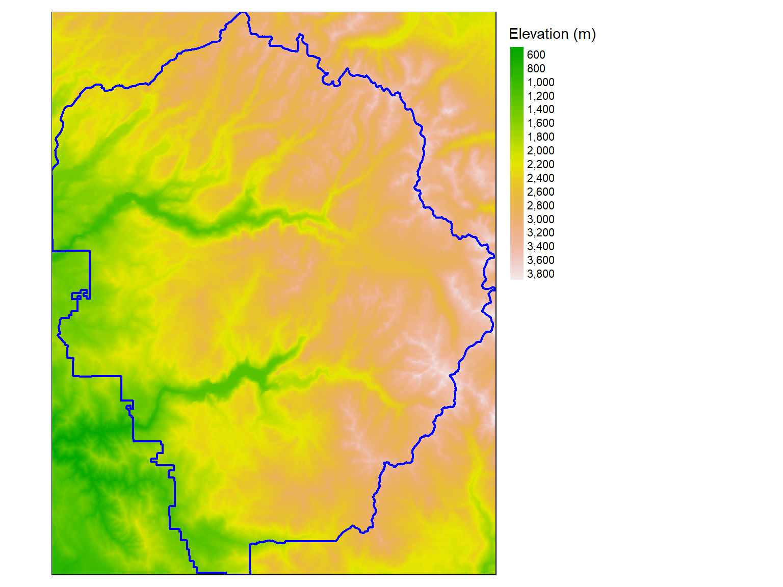

To customize the colors tm_raster() uses, use the arguments n (number of legend elements) and palette (a named palette or vector of color values). Ex:

tm_raster(my_raster, n=10, palette = heat.colors(10))

To plot rasters with continuous values, let style = 'cont'.

Multi-layer rasters can be plotted with tm_rgb(). This function takes arguments r, g, and b to specify how layers should be assigned to red, green, and blue.

Map Elements

Additional map elements like scale bars and north arrows can be added by tacking on additional functions. View the help pages to see the options.

Element	Add with function
Grid lines / tick marks	tm_grid()
Scale bar	tm_scale_bar()
Compass (north arrow)	tm_compass()
Credits text	tm_credits()
Logo	tm_logo()
Axis labels	tm_xlab(), tm_ylab()
Minimap (view mode only)	tm_minimap()

Example: Add a scale bar and compass to the map.

tm_shape(yose_bnd_ll) + 
  tm_polygons(col = "ivory") + 
tm_shape(yose_hp_ll) + 
  tm_symbols(size=0.5, col="forestgreen") +
tm_shape(yose_roads_utm) +
  tm_lines(col="gray60", lwd=1.5, lty="dotted") +
tm_scale_bar(position=c("right", "bottom")) +
tm_compass(position=c("left", "bottom"))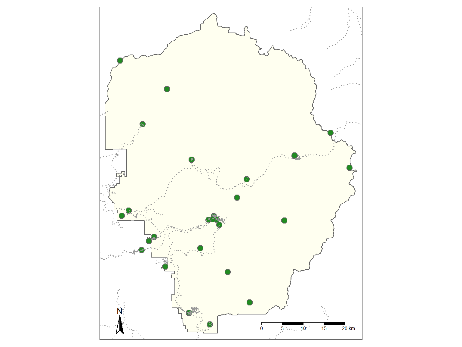

Map element like these are known as ‘Attribute Layers’. In other words they’re treated like layers in terms of stacking, etc.

Global Map Properties

A tmap object can have many other ‘global’ properties, such as the title, size and appearance of the frame, margins, background color, location of the legend, etc.

Enter these with tm_layout(). This function has dozens of arguments you can use.

tm_style(), tm_format(), and tm_legend() are convenience functions that accept subsets of the arguments in tm_layout().

Example: Add a title and change the background color to the YNP map

tm_shape(yose_bnd_ll) + 
  tm_polygons(col = "ivory") + 
tm_shape(yose_hp_ll) + 
  tm_symbols(size=0.5, col="forestgreen") +
tm_shape(yose_roads_utm) +
  tm_lines(col="gray60", lwd=1.5, lty="dotted") +
tm_scale_bar(position=c("right", "bottom")) +
tm_compass(position=c("left", "bottom")) +
tm_layout(main.title = "Yosemite Historic Places", 
          main.title.color = "white",
          bg.color = "darkolivegreen",
          frame = FALSE, 
          attr.color = "white")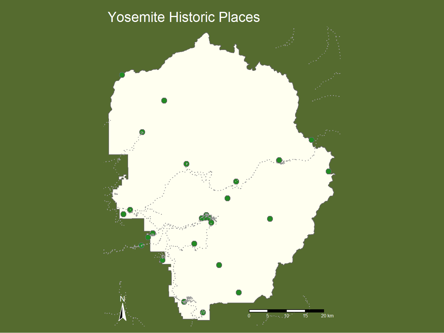

Preset Styles and Formats

tmap supports of handful of predefined styles (symbology) and formats (map layouts, margins, etc.). You can apply these presets using tm_style() and tm_format().

Predefined Styles:

Style	Desc
white	White background, commonly used colors (default)
gray	Grey background, useful to highlight sequential palettes
natural	Emulation of natural view: blue waters and green land
bw	Greyscale, useful for greyscale printing
classic	Classic styled maps
cobalt	Inspired by latex beamer style cobalt
albatross	Inspired by latex beamer style albatross
beaver	Inspired by latex beamer style beaver

Predefined Formats:

Format	Desc
World	Format specified for world maps
World_wide	Format specified for world maps with more space for the legend
NLD	Format specified for maps of the Netherlands

To generate a preview of all of the named Style presets, run the following. This will create a folder of PNG files in the current working directory.

tmap_mode("plot")
tmap_style_catalog()

To assign a named preset style or format for all tmap objects in the current session, use tmap_style() and tmap_format().

Example: Plot the Yosemite Map using the ‘classic’ style preset

tm_shape(yose_bnd_ll) +                             ## Define first layer data source
  tm_polygons() +                                   ## Add features from the source 
tm_shape(yose_hp_ll) +                              ## Add another source (layer)
  tm_symbols(size=0.5) +                            ## Throw on point symbols
tm_shape(yose_roads_utm) +                          ## Add still another source (layer)
  tm_lines(lty="dotted") +                          ## Add lines
tm_scale_bar(position=c("right", "bottom")) +       ## Global element - scale bar
tm_compass(position=c("left", "bottom")) +          ## Global element - north arrow
tm_style("classic") +                               ## Global style preset (default colors)
tm_layout(main.title = "Yosemite Historic Places")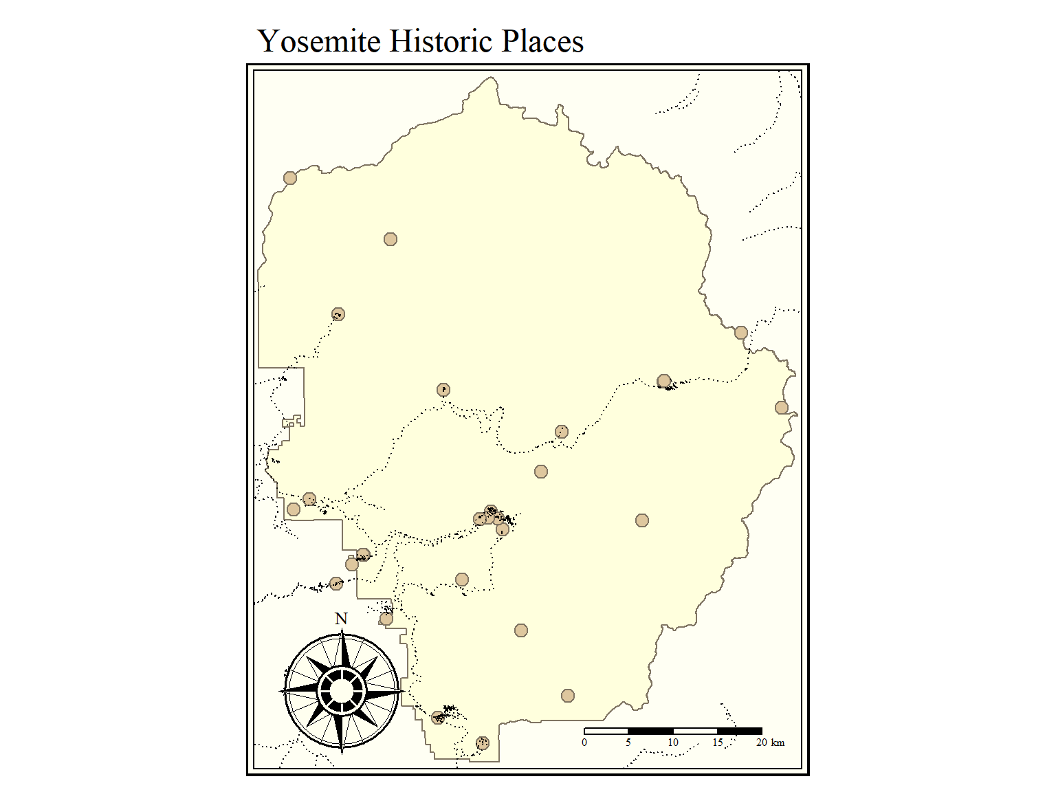

for more tmap tips, run tmap_tip()

R Notebook Exercise

nb_tmap_scgis21.Rmd
Make a map of Yosemite, including the roads, cell towers, and campgrounds

preview notebook | answer key

Interactive Maps

A tmap object can also be rendered as an interactive leaflet map.

Just change the ‘mode’, and redraw the map (by entering the expression at the console).

tmap_mode("view")

## Change to interactive mode
tmap_mode("view")

## tmap mode set to interactive viewing

## Redraw the map (a leaflet window should open)
tm_shape(yose_bnd_ll) + 
  tm_polygons(col = "ivory", alpha=0.5) + 
  tm_shape(yose_hp_ll, size=0.5) + 
  tm_symbols(col="forestgreen")

Interactive leaflet maps work best for small to medium sized datasets. Large datasets and complex features don’t render well as interactive maps.

If needed, tmap will (un)project spatial layers on the fly to geographic coordinates to make them compatible with leaflet.

All of the spatial data in a leaflet is saved in the HTML file. You can minimize the size of the HTML file by removing unneeded attribute columns in your spatial layers.

Most map elements (like compasses, scale bar, etc.) are not supported in interactive maps. For best results keep the design basic.

To re-draw the last map, run tmap_last()

To go back to creating static maps, run tmap_mode("plot")

Basemaps & Popups

tmap’s interactive mode also supports basemap tiles by adding tm_basemap() to your map object.

Customize the Basemap

Change the basemap to "Esri.NatGeoWorldMap":

## Use a custom basemap
tm_shape(yose_bnd_ll) + 
  tm_basemap("Esri.NatGeoWorldMap") + 
  tm_polygons(col = "goldenrod", alpha=0.2) + 
  tm_shape(yose_hp_ll, size=0.5) + 
  tm_symbols(col="forestgreen")

To see a list of tile providers, view the built-in constant leaflet::providers. Previews for most basemap options are available here.

Tiles only work in interactive mode. To add a background to a static map, there’s a workaround using the read_osm() from the tmaptools package. See also the ggmap and ggspatial packages.

Customize the Historic Places Pop-ups

You can specify which attribute values should be displayed with the popup.vars argument. Example:

## Add Change the 
tm_shape(yose_bnd_ll) + 
  tm_basemap("Esri.WorldImagery") + 
  tm_borders(col = "seashell", lwd=2) + 
  tm_shape(yose_hp_ll, size=0.5) + 
  tm_symbols(col="lightgoldenrod", popup.vars = "Name")

To disable popups, set popup.vars = FALSE.

If you need custom HTML in your popup windows, use the leaflet package instead.

Saving and Sharing tmaps

Saving tmap objects as R objects

Like any other R object, tmap objects can be saved to a variable. This allows you to save them to disk using the basic save():

yose_tmap <- tm_shape(yose_bnd_ll) + 
  tm_basemap("Esri.WorldImagery") + 
  tm_borders(col = "seashell", lwd=2) + 
  tm_shape(yose_hp_ll, size=0.5) + 
  tm_symbols(col="lightgoldenrod", popup.vars = "Name")

save(yose_tmap, file = "my_tmap_ynp.RData")

A tmap object with the base layers can be used as a template for other tmap objects. Example:

## Create a tmap object with just the park boundary
ynp_base_tmap <- tm_shape(yose_bnd_ll) + tm_polygons()

## Create a new tmap that builds upon the base and adds the historic points
hp_tmap <- ynp_base_tmap + 
  tm_shape(yose_hp_ll) + 
  tm_symbols()

## Create another one with the roads
roads_tmap <- ynp_base_tmap + 
  tm_shape(yose_roads_utm) +
  tm_lines()

To display a tmap that’s been saved as a variable, type the variable name by itself at the console or use print().

Saving tmap objects as image or HTML files

tmap_save() can be used to save a tmap object as a graphic file (e.g., PNG) or HTML. Example:

yose_tmap <- tm_shape(yose_bnd_ll) + 
  tm_basemap("Esri.WorldImagery") + 
  tm_borders(col = "seashell", lwd=2) + 
  tm_shape(yose_hp_ll, size=0.5) + 
  tm_symbols(col="lightgoldenrod", popup.vars = "Name")

tmap_save(yose_tmap, filename="yose_tmap_test.html")

tmap_save(yose_tmap, filename="~yose_tmap_test.png")

Static maps can be saved as PNG, PDF, EPS, SVG, JPG, BMP, and TIFF files.

You can also use the Export button on the RStudio plot window.

Basemaps are not exported when exporting to image files, and map elements like scale bars are not supported when exporting to HTML.

RPubs is a free service from RStudio for sharing documents on the web. You can publish interactive maps to RPubs by clicking the Publish button on the RStudio Viewer pane.

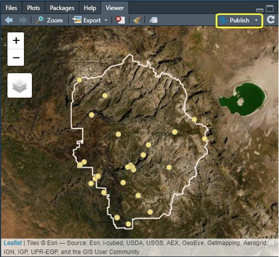
Example of a published interactive map: https://rpubs.com/ajlyons/ynp_historic-places_tmap

Everything published to RPubs is public, so only publish documents that can be viewed by anyone.

leaflet

The leaflet R mapping package provides more ways to customize an interactive map than tmap.

Like tmap, leaflet lets you save interactive maps as stand-alone HTML files (using the leaflet JavaScript library in the background).

Let’s make an interactive map with leaflet package.

library(leaflet)

## Create the map definition with piping syntax
myleaf_map <- leaflet(yose_bnd_ll) %>% addTiles() %>% 
                      addPolygons(data=yose_bnd_ll, fillOpacity=0.1) %>%
                      addCircles(data=yose_hp_ll, popup=~Name)

## Warning: sf layer has inconsistent datum (+proj=longlat +datum=NAD83 +no_defs).
## Need '+proj=longlat +datum=WGS84'

## Show the map
myleaf_map

Caveats for using leaflet

All layers in a leaflet map must be in unprojected geographic coordinates with the WGS84 datum. leaflet does not reproject on the fly!

leaflet runs entirely on the client (browser). This means all spatial data is encoded in the HTML file (with the exception of the basemap tiles). This works fine for small and medium sized spatial data, but not large datasets.

`leaflet` options

leaflet has a lot of other options. You can:

group layers in your leaflet map to turn on and off
tell it to cluster points close together as a single dot that splits aparts as you zoom in
fine-tune popup windows with HTML code
use JavaScript add-ons

For more info, see:

Leaflet for R. RStudio

WebMaps in R with Leaflet. Patty Frontiera

Spatial Data Analysis with R
Society for Conservation GIS, July 2021

`tmap`

Building a Map with `tmap`

tmap layers

Example: A One-Layer Map

Multi-layered maps

Reprojection on the Fly

Example

Symbology

Symbolizing by Attribute Value

Example: Use a different color for each road type

Tweaking the Legend

Anatomy of a Choropleth Map in `tmap`

Example: Map Population by County

Raster Layers

Example: Plot the DEM for Yosemite

Map Elements

Example: Add a scale bar and compass to the map.

Global Map Properties

Example: Add a title and change the background color to the YNP map

Preset Styles and Formats

Example: Plot the Yosemite Map using the ‘classic’ style preset

R Notebook Exercise

Interactive Maps

Basemaps & Popups

Customize the Basemap

Customize the Historic Places Pop-ups

leaflet

Caveats for using leaflet

`leaflet` options

Summary

Spatial Data Analysis with R Society for Conservation GIS, July 2021

tmap

Building a Map with tmap

tmap layers

Example: A One-Layer Map

Multi-layered maps

Reprojection on the Fly

Example

Symbology

Symbolizing by Attribute Value

Example: Use a different color for each road type

Tweaking the Legend

Anatomy of a Choropleth Map in tmap

Example: Map Population by County

Raster Layers

Example: Plot the DEM for Yosemite

Map Elements

Example: Add a scale bar and compass to the map.

Global Map Properties

Example: Add a title and change the background color to the YNP map

Preset Styles and Formats

Example: Plot the Yosemite Map using the ‘classic’ style preset

R Notebook Exercise

Interactive Maps

Basemaps & Popups

Customize the Basemap

Customize the Historic Places Pop-ups

Saving and Sharing tmaps

Saving tmap objects as R objects

Saving tmap objects as image or HTML files

Sharing Interactive Maps with RPubs

leaflet

Caveats for using leaflet

leaflet options

Summary

Spatial Data Analysis with R
Society for Conservation GIS, July 2021

`tmap`

Building a Map with `tmap`

Anatomy of a Choropleth Map in `tmap`

`leaflet` options