Intro to Spatial Data Analysis with R
SCGIS 2023 Annual Conference

Getting Started with R & RStudio

R and RStudio

Why is R So Popular?

It’s free!
Huge user community (especially academics)
Thousands of add-ons (packages) that extend its capabilities
Particularly strong in plotting and reporting
Strong on spatial data
Once you get over the initial hump, can work very efficiently
Makes it easy to get your code “out there”
Solid overall programming language

a programming language to write scripts
software (“environment”) that interprets scripts written in R
inspired by ‘S’ (1976), first beta version ~2000
lots of user-contributed packages:
- CRAN: >24,500
- Bioconductor: >2,100
- R-Forge: >2,200
- GitHub: >85,500

a very popular tool (IDE) to work with both R software and R scripts
Version 1.0 came out in late 2016
has lots of convenience functions
RStudio needs R to run, but you can use R without RStudio

formerly known as RStudio Cloud
online RStudio and Jupyter Notebooks
requires an account (free account gets you 25 hrs / month)
98% same as RStudio Desktop
have to upload your data to the cloud
everything gets saved between sessions
workspaces and projects can be shared with collaborators

Exercise 1: RStudio Exploration and Basic Commands

Exercise 1 Topics

Using R like a fancy calculator
Order of operations
Comparison operators
Saving the results of expressions to variable
Rules for naming variables

RStudio Cloud project for this workshop:

https://posit.cloud/content/6309720

After it opens, click on ‘Save a Permanent Copy’:

Break!

Exercise 1 Review

Key vocabulary terms are in italic.

When you enter an expression at the console, R will evaluate the expression, and print the results at the console.
If you enter an incomplete expression, R will prompt you to finish the job by showing a ‘+’ symbol in the console
You can save the results of an expression to an object (variable) using an assignment operator
=
<-
R objects can be named almost anything (but no spaces or hyphens please)
R is case sensitive about everything
Once defined, R objects can be used in subsequent expressions
R objects can be updated (assigned a new value)
R objects are only saved in memory, and will disappear when you close RStudio
Comparison operators return TRUE or FALSE (aka Logical values)

> >= < <= ==

R has a few built-in constants, which are like objects but you don’t have to define them

Naming Objects

The rules for naming objects are pretty flexible. You can use numbers, letters, and most special characters.

A few rules to take note of:

Can’t start with a number: 3pieces
Hyphens and spaces not allowed: first name, last-name
Don’t use the name of a built-in function, constant, or keyword: c, pi

Naming Styles

There are a handful of popular naming styles. Pick one that you like, and be consistent!

Style	Example
alllowercase	adjustcolor
period.separated	shoe.size
underscore_separated (aka snake case)	numeric_version
lowerCamelCase	addTaskCallback
UpperCamelCase	SignatureMethod

Data Types

All variables have a class or data type, which you can view using class().

num_plots = 10
class(num_plots)

## [1] "numeric"

Other common data types:

character
factor
date
data frame, tibble
matrix
list

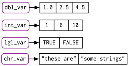
Vectors

vectors are R objects that contain multiple values of the same class.

Example:

i = 4:12
i

## [1]  4  5  6  7  8  9 10 11 12

More examples:

Creating Vectors

In general, you need to use a function or operator to create a vector.

Sequence of numbers with the : operator:

1:10

##  [1]  1  2  3  4  5  6  7  8  9 10

Repeat function:

rep("Quercus lobata", 5)

## [1] "Quercus lobata" "Quercus lobata" "Quercus lobata" "Quercus lobata" "Quercus lobata"

Combine elements of the same class with c():

yn <- c(TRUE, FALSE, TRUE)
yn

## [1]  TRUE FALSE  TRUE

Some built-in constants are also vectors:

LETTERS

##  [1] "A" "B" "C" "D" "E" "F" "G" "H" "I" "J" "K" "L" "M" "N" "O" "P" "Q" "R" "S" "T" "U" "V" "W" "X" "Y" "Z"

state.abb

##  [1] "AL" "AK" "AZ" "AR" "CA" "CO" "CT" "DE" "FL" "GA" "HI" "ID" "IL" "IN" "IA" "KS" "KY" "LA" "ME" "MD" "MA" "MI" "MN" "MS" "MO" "MT"
## [27] "NE" "NV" "NH" "NJ" "NM" "NY" "NC" "ND" "OH" "OK" "OR" "PA" "RI" "SC" "SD" "TN" "TX" "UT" "VT" "VA" "WA" "WV" "WI" "WY"

month.name

##  [1] "January"   "February"  "March"     "April"     "May"       "June"      "July"      "August"    "September" "October"   "November" 
## [12] "December"

Random number functions:

runif(20)

##  [1] 0.47222650 0.32177990 0.47102296 0.31255999 0.37411543 0.83883019 0.54412414 0.79563818 0.86056624 0.37776087 0.13241074 0.04561497
## [13] 0.12573181 0.35008028 0.10085344 0.24164384 0.88692435 0.58348380 0.40103117 0.05853828

rnorm(20)

##  [1]  0.17259189  1.05045045 -0.77576319  0.38853854  1.21766611 -0.44178341 -0.49117499  0.45152488 -1.00500504 -0.28446580 -0.47148116
## [12]  0.67110532  1.10437365 -0.08966662 -0.32382897 -0.35828034  1.35148125  0.70476880 -0.31489782 -0.85387276

sample(month.abb, 3)

## [1] "Jan" "May" "Jun"

How Vectors Behave

Vectorized operations

Many R functions and math operators are vectorized (i.e., operate on each individual element).

Examples

First we create two numeric vectors:

x = 0:4
x

## [1] 0 1 2 3 4

y = 11:15
y

## [1] 11 12 13 14 15

Are sin() & cos() vectorized?

sin(x)

## [1]  0.0000000  0.8414710  0.9092974  0.1411200 -0.7568025

cos(x)

## [1]  1.0000000  0.5403023 -0.4161468 -0.9899925 -0.6536436

Addition (and all math functions) is vectorized:

x + 1

## [1] 1 2 3 4 5

x + y

## [1] 11 13 15 17 19

Aggregate functions

Functions that accept a vector and spit out a single value are aggregate.

x = runif(20)
x

##  [1] 0.19164316 0.14713477 0.52358202 0.36361698 0.66091639 0.89028906 0.50335611 0.02837383 0.27831807 0.04872274 0.90151351 0.47016136
## [13] 0.87231665 0.52445658 0.30225813 0.67669765 0.39608536 0.06927169 0.64936000 0.45437898

Most descriptive stats functions are aggregate:

mean(x)

## [1] 0.4476227

median(x)

## [1] 0.4622702

sd(x)

## [1] 0.2743128

Other aggregate functions:

first(state.name)

## [1] "Alabama"

Subsetting Vectors

To extract a single element from a vector, use square bracket notation. Inside the square brackets, put the index of the element(s) you want.

Subset with indices

LETTERS[2]

## [1] "B"

To return multiple elements, pass a vector of indices.

LETTERS[2:4]

## [1] "B" "C" "D"

You can also use square brackets to extract elements in a different order.

LETTERS[4:2]

## [1] "D" "C" "B"

Subset with logicals

You can also insert a vector of Logical values (TRUE/FALSE) in the brackets. R will return the corresponding element for the TRUE values.

LETTERS[c(T,T,T,T,T,T,T,T,F,F,F,F,F,F,F,F,F,F,F,F,F,F,F,F,F,F)]

## [1] "A" "B" "C" "D" "E" "F" "G" "H"

Better still, use an expression that returns a vector of logical values:

state.abb[ substr(state.abb, 1, 1) == "N" ]

## [1] "NE" "NV" "NH" "NJ" "NM" "NY" "NC" "ND"

Exercise 2: Working with Scripts and Vectors

Exercise 2 Topics

Saving code in scripts
Data types
Vectors

Exercise 2 Review

vectors are R objects that contain multiple values of the same class
Some functions that return vectors:
c() seq() rnorm() sample()
You can build vectors from scratch using: c()
Functions and operators that operate on each element of a vector and return another vector are said to be vectorized

round(), abs() + - * /
Functions that take multiple elements of a vector and spit out a single value are said to be aggregate functions

sum(), min(), mean(), max()
You can plot the distribution of numeric data using plotting functions like:

hist(), boxplot(), plot()

Scripts

Top five advantages of using scripts over the console:

Easier to write (and fix!) your code
You can add comments to remind yourself what each command is doing
Reuse your own code
You can add loops and if-then statements later on
Tell your friends you’re a coder!

Intro to Spatial Data Analysis with R SCGIS 2023 Annual Conference