How to Import CA Groundwater Basins into R with arcgislayers
Summary
The notebook demonstrates how to import the DWR Groundwater Basins 2016 layer into R, using the arcgislayers package. We will also extract one of the basins and save it to a geojson file.
Locate the Data
First, we need to find the data. A Google Search of “CA Groundwater Basins GIS Data” quickly gets us to a list of groundwater layers hosted by CA DWR. Select one of the layers and view the full details. The “View Data Source” button gets us to the MapServer page for this map.
The layer from this MapServer have been made public, so we should be able to download it fairly easily. If it wasn’t public, but we had an ArcGIS account that gave us permission to view it, we could still get it after authenticating with arcgislayers.
Setup
Next, load the packages we’ll need:
Connect to the MapServer
The general sequence of steps to import data from ArcGIS servers using arcgislayers is
- authenticate (if needed)
- create a connection to the MapServer or FeatureServer that has the data
- list the FeatureLayers available
- create a connection to the desired FeatureLayer
- view the fields in the FeatureLayer (optional - if you want to construct a WHERE query when you import the data)
- import the data
First, we open a connection to the MapServer.
grndwtr_basins2016_url <- "https://gispublic.waterboards.ca.gov/portalserver/rest/services/GAMA/DWR_Groundwater_Basins_2016/MapServer"
grndwtr_basins2016_ms <- arc_open(grndwtr_basins2016_url)
grndwtr_basins2016_ms
<MapServer <1 layer, 0 tables>>
CRS: 3857
Capabilities: Map,Query,Data
0: DWR Groundwater Basins 2016 (esriGeometryPolygon)ArcGIS MapServers and FeatureServers are both set up to share multiple layers. So next, we view which FeatureLayer(s) this MapServer contains:
list_items(grndwtr_basins2016_ms)After taking note of the id of the layer we want to import, we can now create a connection to the FeatureLayer provided by this MapServer. (Note this still isn’t importing the data, just creating the connection):
grndwtr_basins2016_fl <- get_layer(grndwtr_basins2016_ms, id = 0)
grndwtr_basins2016_fl
<FeatureLayer>
Name: DWR Groundwater Basins 2016
Geometry Type: esriGeometryPolygon
CRS: 3857
Capabilities: Map,Query,DataNow that we have the FeatureLayer object, we can look at the fields in the attribute table. This could be useful if for example we wanted to create a WHERE expression when we import the data.
list_fields(grndwtr_basins2016_fl)Import the Spatial Data
Up to now, all we’ve done is open connections to the data on DWR’s ArcGIS Server. This is a bit like dialing a phone number and saying hello. We haven’t yet actually imported any spatial data into R.
Finally, we have everything we need import the data using arc_select(). This function imports the layer and returns it as a simple feature (sf) object. It has optional arguments to specify attribute and/or spatial conditions, which can be extremely helpful with large datasets, but we don’t need that here.
grndwtr_basins2016_sf <- arc_select(grndwtr_basins2016_fl)Registered S3 method overwritten by 'jsonify':
method from
print.json jsonlitegrndwtr_basins2016_sfSimple feature collection with 517 features and 7 fields
Geometry type: POLYGON
Dimension: XY
Bounding box: xmin: -13843560 ymin: 3833624 xmax: -12715550 ymax: 5161543
Projected CRS: WGS 84 / Pseudo-Mercator
First 10 features:
FID basin_id basin_subb basin_su_1 basin_name subbasin_n region_off
1 0 2-036 2-036 2-36 SAN PEDRO VALLEY NCRO
2 1 2-011 2-011 2-11 SUNOL VALLEY NCRO
3 2 6-014 6-014 6-14 FISH LAKE VALLEY SRO
4 3 2-008 2-008 2-08 CASTRO VALLEY NCRO
5 4 2-032 2-032 2-32 VISITACION VALLEY NCRO
6 5 2-037 2-037 2-37 SOUTH SAN FRANCISCO NCRO
7 6 5-069 5-069 5-69 YOSEMITE VALLEY SCRO
8 7 6-011 6-011 6-11 LONG VALLEY SRO
9 8 2-033 2-033 2-33 ISLAIS VALLEY NCRO
10 9 2-010 2-010 2-10 LIVERMORE VALLEY NCRO
geometry
1 POLYGON ((-13634455 4520706...
2 POLYGON ((-13569437 4528443...
3 POLYGON ((-13111604 4488036...
4 POLYGON ((-13589440 4532332...
5 POLYGON ((-13624018 4538528...
6 POLYGON ((-13620816 4540890...
7 POLYGON ((-13304977 4546014...
8 POLYGON ((-13237363 4546707...
9 POLYGON ((-13623559 4544912...
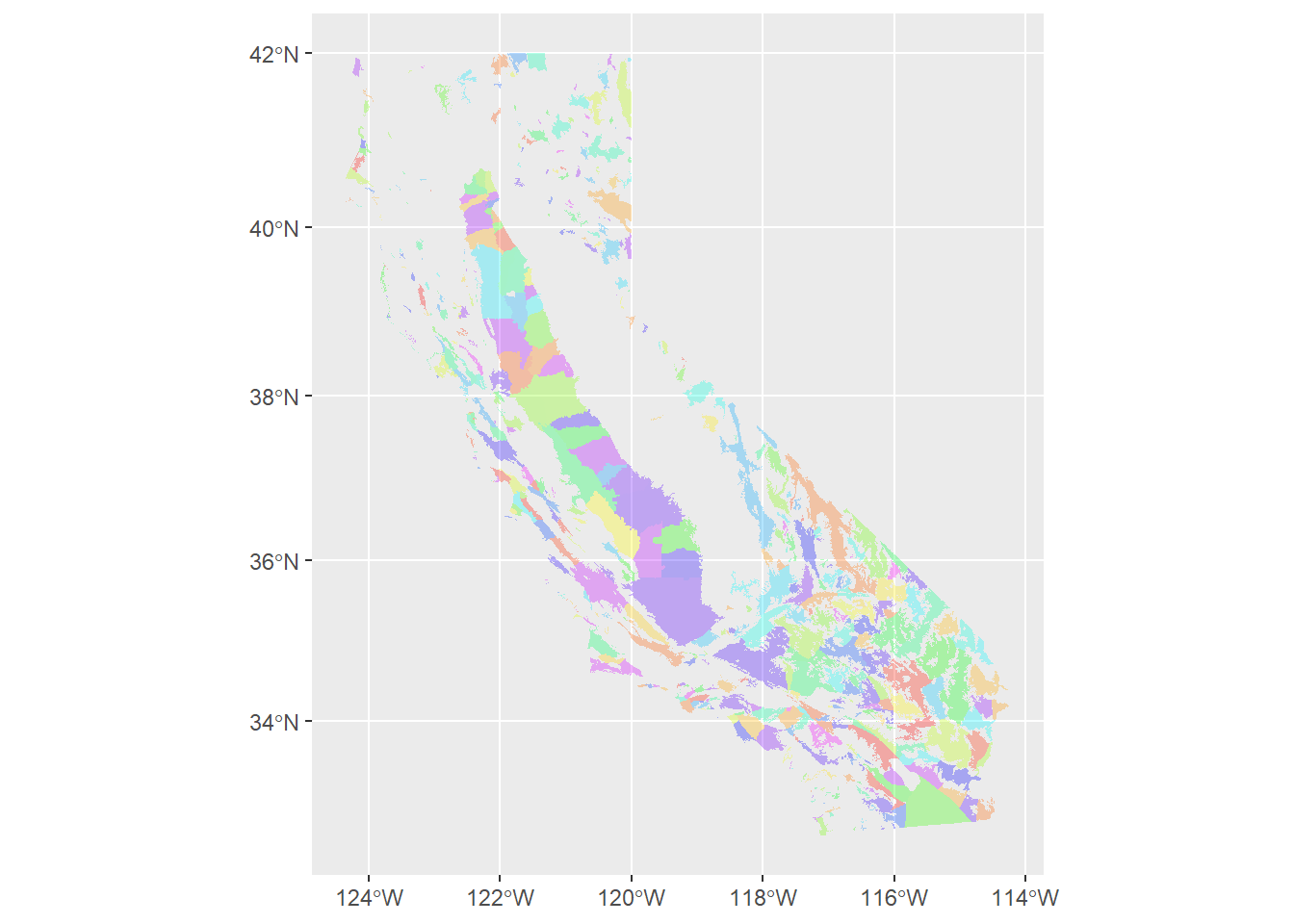
10 POLYGON ((-13557839 4525079...We now have the polygons as a sf object! Let’s create a column of unique colors, and map them:
Export One Basin to Disk
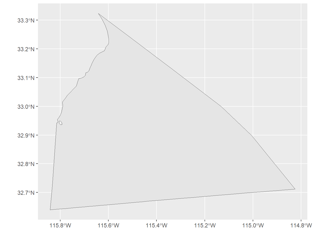
Pull out the groundwater basin for Imperial Valley, and plot it:
impval_2016_sf <- grndwtr_basins2016_sf |>
  filter(basin_name == "IMPERIAL VALLEY")

ggplot() + geom_sf(data = impval_2016_sf)
Convert it to geographic coordinates, and save as geojson:
st_write(impval_2016_sf |> st_transform(4326),
         dsn = "imperial-valley-groundwater-basin-2016.geojson",
         delete_dsn = TRUE)
Deleting source `imperial-valley-groundwater-basin-2016.geojson' using driver `GeoJSON'
Writing layer `imperial-valley-groundwater-basin-2016' to data source
`imperial-valley-groundwater-basin-2016.geojson' using driver `GeoJSON'
Writing 1 features with 8 fields and geometry type Polygon.