

IGIS Tech Notes describe workflows and techniques for using geospatial science and technologies in research and extension. They are works in progress, and we welcome feedback and comments.
Background
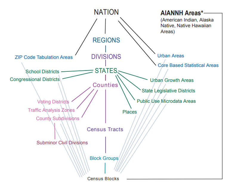
Most people know the US Census Bureau tabulates their data by Census Blocks, which are then aggregated into Block Groups and Tracks, as their primary enumeration areas. Not as many people know the Census Bureau also maintains GIS data for many other administrative boundaries, which they use to produce thousands of different data summaries. This collection of authoritative administrative spatial data can be downloaded for free, and is a tremendous resource you can use in any GIS project!
In this Tech Note, we’ll show you how to download administrative
boundaries via the tigris
R package by Kyle Walker. tigris has a number of
convenience functions to import different census geographies into R via
the Census API (you don’t need an API key to download the spatial data).
The functions you can use include:
blocks()
block_groups()
tracts()
counties()
states()
regions()
places()
pumas()
school_districts()
zctas()
urban_areas()
metro_divisions()
county_subdivisions()
congressional_districts()
state_legislative_districts()
voting_districts()
native_areas()
landmarks()
military()
primary_roads()
primary_secondary_roads()
roads()
rails()
All of these functions bring the spatial data into R as sf objects by
default. (If you want tp keep the Shapefiles as well, you can set the
keep_zipped_shapefile argument to TRUE.) For
full details, view the function help pages.
Pro Tip: If you want to download not just the spatial data but also data from the decennial census or American Community Survey, see the tidycensus package.
Example: Import Incorporated California Cities and Towns
In this example, we’ll import the the boundaries of incorporated
cities and towns in California using tigris.
1. Load packages:
Step 1 is to load the packages we’ll need:
library(tigris)
library(dplyr)
library(sf)
library(leaflet)
Set Tigris cache option:
options(tigris_use_cache = TRUE)
2. Get the Places Dataset
Incorporated cities and towns are part of the Places
dataset, which we can download via places().
ca_places_sf <- places(state = "CA", cb = FALSE, progress_bar = FALSE) |> st_transform(4326)## Retrieving data for the year 2021dim(ca_places_sf)## [1] 1611 17head(ca_places_sf)## Simple feature collection with 6 features and 16 fields
## Geometry type: MULTIPOLYGON
## Dimension: XY
## Bounding box: xmin: -120.6741 ymin: 33.62517 xmax: -117.6746 ymax: 40.45356
## Geodetic CRS: WGS 84
## STATEFP PLACEFP PLACENS GEOID NAME NAMELSAD LSAD CLASSFP
## 1 06 77364 02412017 0677364 Susanville Susanville city 25 C1
## 2 06 02000 02409704 0602000 Anaheim Anaheim city 25 C1
## 3 06 16532 02410239 0616532 Costa Mesa Costa Mesa city 25 C1
## 4 06 17750 02410282 0617750 Cypress Cypress city 25 C1
## 5 06 28000 02410556 0628000 Fullerton Fullerton city 25 C1
## 6 06 29000 02410568 0629000 Garden Grove Garden Grove city 25 C1
## PCICBSA PCINECTA MTFCC FUNCSTAT ALAND AWATER INTPTLAT INTPTLON
## 1 Y N G4110 A 20507839 218688 +40.4336740 -120.6283062
## 2 Y N G4110 A 130206498 1567025 +33.8555018 -117.7586572
## 3 Y N G4110 A 40937896 24554 +33.6659055 -117.9123358
## 4 N N G4110 A 17128118 22347 +33.8184768 -118.0383074
## 5 N N G4110 A 58065841 32825 +33.8857156 -117.9280247
## 6 N N G4110 A 46520862 31066 +33.7787816 -117.9604719
## geometry
## 1 MULTIPOLYGON (((-120.5261 4...
## 2 MULTIPOLYGON (((-118.0175 3...
## 3 MULTIPOLYGON (((-117.9546 3...
## 4 MULTIPOLYGON (((-118.0633 3...
## 5 MULTIPOLYGON (((-117.9854 3...
## 6 MULTIPOLYGON (((-118.0429 3...
Reading the docs, we see that the Places dataset contains all sorts
of stuff. But we can use the LSAD column (Legal/Statistical
Area Description) to pull out just the incorporated cities and towns.
Let see what it contains:
ca_places_sf$LSAD |> table()##
## 25 43 57
## 461 21 1129
Looking up the LSAD codes, we find:
25. City (suffix). Consolidated City, County or Equivalent Feature, County Subdivision, Economic Census Place, Incorporated Place
43. Town (suffix). County Subdivision, Economic Census Place, Incorporated Place
57. CDP (suffix). Census Designated Place, Economic Census Place (not incorporated)
Therefore, we want the Places where the LSAD is 25 (cities) or 43 (towns):
ca_cities_towns_sf <- ca_places_sf |>
filter(LSAD %in% c(25, 43))
dim(ca_cities_towns_sf)## [1] 482 17
3. Plot the Data to Cross-Check
Plotting is a good way to reality-check the data. First we download the state boundary:
cabnd_sf <- states(cb = TRUE) |> filter(GEOID == "06") |> st_transform(4326)## Retrieving data for the year 2021
Next, we make a version of the cities & towns layer that includes a column of color values:
random_cols <- c("#89C5DA", "#DA5724", "#74D944", "#CE50CA", "#3F4921", "#C0717C", "#CBD588", "#5F7FC7", "#673770", "#D3D93E", "#38333E", "#508578", "#D7C1B1", "#689030", "#AD6F3B", "#CD9BCD", "#D14285", "#6DDE88", "#652926", "#7FDCC0", "#C84248", "#8569D5", "#5E738F", "#D1A33D", "#8A7C64", "#599861")
ca_cities_towns_4map_sf <- ca_cities_towns_sf |>
mutate(col = sample(random_cols, nrow(ca_cities_towns_sf), replace = TRUE)) |>
select(NAMELSAD, col)
Now we can make the plot in leaflet:
leaflet(cabnd_sf) |>
addProviderTiles("CartoDB.Positron") |>
addPolygons(fill = FALSE, color = "black", weight = 5) |>
addPolygons(data = ca_cities_towns_4map_sf, color = "#777", weight = 1,
fill = TRUE, fillColor = ~col, popup = ~NAMELSAD)Looks good!
4. Export as CSV and GeoJSON
The layers we’ve imported are standard simple feature data frames, so
we can export them to disk using write.csv() for just the
attribute table, or st_write() to save the data in various
GIS file formats.
Save the attribute table as a CSV file:
ca_cities_towns_sf |>
select(GEOID, NAME, LSAD, LAND_AREA_M2 = ALAND, WATER_AREA_M2 = AWATER) |>
st_drop_geometry() |>
write.csv(file = "./outputs/ca_cities_towns_2021.csv", row.names = FALSE)You can preview and download the CSV file here.
Save the spatial data with a handful of columns as GeoJSON:
ca_cities_towns_sf |>
select(GEOID, NAME, LSAD, LAND_AREA_M2 = ALAND, WATER_AREA_M2 = AWATER) |>
st_write(dsn = "./outputs/ca_cities_towns_2021.geojson", delete_dsn = TRUE)## Deleting source `./outputs/ca_cities_towns_2021.geojson' using driver `GeoJSON'
## Writing layer `ca_cities_towns_2021' to data source
## `./outputs/ca_cities_towns_2021.geojson' using driver `GeoJSON'
## Writing 482 features with 5 fields and geometry type Multi Polygon.You can preview and download the GeoJSON file here.
Summary
The US Census Bureau is a great source of up-to-date spatial data for
many types of administrative boundaries for the USA. You can import
these data into R fairly easily with the tigris package,
and then use functions from dplyr and sf to
wrangle the data and export them as GIS files. This is a great resource
for any GIS project.
This work was supported by the USDA - National Institute of Food and Agriculture (Hatch Project 1015742; Powers).
