IGIS Tech Notes describe workflows and techniques or using geospatial science and technologies in research and extension. They are works in progress, and we welcome feedback and comments.

Background

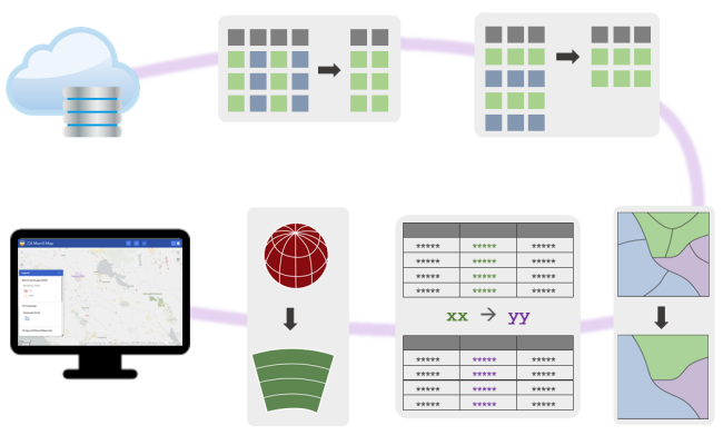
Web maps commonly include reference GIS layers, such as property boundaries, administrative areas, infrastructure features, etc. Such reference layers are often maintained by an organization such as a government agency, research unit, land owner, company, etc.

Reference layers are typically not hard to find, because the organizations that maintain generally make them publicly available. That being said, reference layers often require some manipulations before you can use them in a web map, and like everything else will need updates from time-to-time.

If you’re lucky (or your goals are flexible), you may be able to use a reference layer ‘as-is’. More likely, you may have to do one or more of the following manipulations to get a reference layer ‘ready’ for a web map, depending on how you want the web map to function and what you get from the reference layer.

dissolve simple polygons into multipart polygons based on an attribute
explode multipart polygons into simple polygons
generate text fields for labels and popup windows
omit features
split subsets of features into different layers
remove unneeded fields in the attribute table
compute the area and/or perimeter of featuers in specific units (e.g, acres)
standardize field names
change the capitalization of values in the attribute table
repair invalid geometries
get rid of z-values
project to Web Mercator
create a point version of a polygon layer to be visible when zoomed out

The first step is to determine what needs to be done to get the ‘authoritative’ reference data ready for your web map. This will largely depend on the design and functionality of your web map (see table below for some examples). Once you figure out what you need to do, all of the above can be done using desktop GIS software like ArcGIS Pro or QGIS. Some operations can also be done in your web mapping platforms (like ArcGIS.com).

The pain point however comes when a new version of the authoritative data is released by the publisher. The changes may only be to a small number of features, but if you want your web map to be current you now have to repeat the entire process of transforming the data for your web map. Hopefully you wrote down that sequence of geoprocessing steps you carefully developed 15 months ago? Hopefully it won’t take too long to go through the workflow all over again?

I have to do this again?

Scripting to the Rescue!

This is a good example where scripting can pay off - handsomely. If you do your data prep using a scripting language like R or Python, repeating the processing becomes a whole lot easier. And not only is it easier, you’re also less likely to forget a step. Your web map will thank you!

Scripting is not a panacea for everything, because it almost always takes more time to write code than use a “point and click” tool. But transforming reference layers that you don’t control for a web map that you want to stay current is a use case where scripting makes a whole lot of sense.

The table below shows some of the common operations needed in web mapping, and the corresponding R functions you can use from the sf and dplyr packages. Further below, we’ll see an actual example.

Operation	Use Case	R function(s)
Dissolve simple polygons into multipart polygons	Sometimes multiple simple polygons belong to the same entity (e.g., a park may consist of several pieces of land). In your web map, you may want labels and popups to be associated at the entity level, hence you need to dissolve boundaries based on attribute values.	`dplyr::group_by()` followed by `dplyr::summarise()`
Explode multipart polygons into simple polygons	In some web maps, you might not want multipart polygons. For example, the individual parts of a parent feature may need to be treated independently for intersections or management. Think for example of a county which includes distant islands that are technically part of the county but should be treated as separate areas on your web map.	`st_cast()`
Delete unneeded fields in the attribute table	Most reference datasets have extra fields in the attribute table that you really don’t need in your web map (sometimes there are lots of extra fields!). Getting rid of them reduces overhead, improves performance, and simplifies building the web map.	`dplyr::select()`
Generate text fields for labels and popup windows	Most web platforms give you some ability to customize text for labels and popup windows. This includes basic character formatting, concatenating fields, adding prefixes and punctuation, wrapping text in HTML tags, etc. More complex text manipulation, such as search and replace functions, word swaps, or grabbing text from lookup tables is a lot easier to do in a script.	`dplyr::mutate()` with `paste()` and various functions from the `stringr` package
Filter features	There are many cases where you only need some of the features in a reference layer for your web map. If your preferred features can be idenified via attribute fields, and/or their spatial relationship to your area of interest, it is easy to filter them with your script.	`dplyr::filter()`, `st_intersects()`, `st_disjoint()`, `st_contains()`, etc.
Split subsets of features into different layers	Reference datasets may contain many types or categories of features, that you might want separated in your web map. For example a ‘Places’ layer may contain features for libraries, court houses, schools, fire stations, etc. Splitting these up into separate datasets can make your web map easier to navigate and reduce overhead.	`dplyr::filter()`
Compute area and/or perimeter in specific units	It is not uncommon to get a polygon dataset with a field called ‘Shape_Area’ containing the area in map units. ArcGIS Online will even create this field for you when you upload spatial data. However map units squared are often ginormous numbers not useful on web maps. Computing area in acres, hectares, miles squared, etc. is easy to build into your data processing pieline, and you can even specify the number of decimal places to keep.	`sf::st_area()`, `units::set_units()`, `round()`
Standardize field names	You may find it easier to build your web map if the field names follow a standard naming conventions, particularly if you create custom expressions using Arcade or Javascript. This may involve converting everything to lower case, replacing spaces with underscores, etc.	`stringr::str_to_upper()`, `stringr::str_to_lower()`, `stringr::str_replace()`
Change capitalization	Sometimes you get GIS layers that use ALL CAPS for things like place names, labels, and even comments. You may not want to keep ALL CAPS in your web map, which offer other formatting options to indicate officialness or emphasis.	`stringr::str_to_upper()`, `stringr::str_to_lower()`, `stringr::str_to_title()`
Repair invalid geometries	It is not uncommon to get invalid geometries in vector data, which could include weird overlapping segments of a polygon, slivers smaller than the tolerance level, topology errors, etc. Contact the data producer to let them know, but in the meantime many (but not all) geometries errors can fixed in R.	`sf::st_make_valid()`
Get rid of z-values	It’s not uncommon to get a vector layer with z-values that are all 0. Unless the features are on the surface of the ocean, this usually an error in the production. Even if the z-values are valid, they’re usually not useful for web mapping unless you’re doing 3D rendering. Fortunately they’re easily removed.	`sf::st_zm()`
Project to Web Mercator	Web Mercator is the coordinate reference system for almost all web map platforms (including ERSI). Although your web mapping engine may reproject data to web mercator on the fly, it’s easy enough to build into a pipeline. Plus you’ll be able to control and check the results locally.	`st_transform(3857)`
Create a point version of a polygon layer	Small polgyons are often not visible on a web map when you’re zoomed out. A common workaround is to add an additional point version of the layer (because point layers draw at every scale). The point layer is configured to dislay at small scales (zoomed out), and as the user zooms in the polygon layer appears.	`sf::st_centroid()`

Uploading the Cleaned Up Reference Layer to Your Web Map

After you’ve got the reference layer ready to go, the next step is to upload it to your web mapping platform. This generally involves saving the layer to disk, and then uploading it via the browser.

The best file format for saving the data will vary depending on the web mapping platform. ArcGIS.com supports a number of spatial file formats you can use to upload your data. I would recommend GeoJSON in most cases. GeoJSON is easily exported from R, and ArcGIS.com can create a hosted feature layer without any additional steps or settings.

A couple of caveats about GeoJSON files include:

A single GeoJSON file can only contain one layer (more specifically, the gdal driver that sf and other packages use to write GeoJSON files to disk only supports a single layer per .geojson file).
GeoJSON is a plain text format, This makes it easy to read with any text editor, however it can also result in large files. If your dataset is particularly big, consider thinning it down further or use one of the alternate formats below.
GeoJSON can handle projections. Projecting your layer to Web Mercator (epsg 3857) before you upload it is strongly recommended so this operation doesn’t have to be done on the server.

Other file formats that ArcGIS.com can use as the data source for a hosted feature layer include Shapefiles (zipped) and file geodatabases (zipped).

Example: Preparing REC boundaries for a Web Map

The rest of this Tech Note will work through an example of prepping an authoritative reference layer for a web map using R. In this case, we’ll be making some tweaks to the authoritative boundary layer for Research and Extension Centers (RECs) under the University of California Division of Agriculture and Natural Resources (UCANR).

Import the Authoritative Layer

Step 1 is to import the authoritative reference layer into R. In some cases, this may require downloading a dataset to your hard drive as a Shapefile or file geodatabase. But many organizations are publishing authoritative layers online. In this example, we’ll grab the layer directly from the publisher via an ArcGIS Open Data Hub.

First, we load the libraries we’ll need:

library(sf)
library(dplyr)
library(tmap)
library(units)

First we find the URL to the Feature Service. This make take a little exploring, but keep clicking on links that say “Full Details” and “Data Source” until you see a URL that looks like:

https://geodata.ucanr.edu/arcgis/rest/services/REC_Data/FeatureServer/0

Now we can import it using the R-ArcGIS bridge. Assuming we have an active license to ArcGIS and have installed the package (via ArcGIS Pro), we can load it with:

library(arcgisbinding)

## *** Please call arc.check_product() to define a desktop license.

## verify the license
arc.check_product()

## product: ArcGIS Pro (12.9.3.32739)
## license: Advanced
## version: 1.0.1.300

Now we’re ready to import the data:

recs_bnd_url <- "https://geodata.ucanr.edu/arcgis/rest/services/REC_Data/FeatureServer/0"

## Create a connection object
recs_bnd_con <- arc.open(path = recs_bnd_url)

## Display info (metadata)
recs_bnd_con

## dataset_type    : FeatureClass
## path            : https://geodata.ucanr.edu/arcgis/rest/services/REC_Data/FeatureServer/0 
## fields          : id, acres, shape_leng, name, reports_li, brochure_l, 
## fields          : objectid, globalid, shape
## extent          : xmin=-13703909, ymin=3869281, xmax=-12850582, ymax=5156216
## geometry type   : Polygon
## WKT             : PROJCS["WGS_1984_Web_Mercator_Auxiliary_Sphere",GEOGCS["GCS_...
## WKID            : 3857

Import the features and convert them to sf:

recs_bnd_sf <- arc.select(recs_bnd_con) %>% arc.data2sf()
recs_bnd_sf

## Simple feature collection with 10 features and 8 fields
## Geometry type: GEOMETRY
## Dimension:     XY
## Bounding box:  xmin: -13703910 ymin: 3869281 xmax: -12850580 ymax: 5156216
## Projected CRS: WGS 84 / Pseudo-Mercator
##    id acres shape_leng            name
## 1   1  5677 40036.8435 Sierra Foothill
## 2   2  5289 25136.9868            HREC
## 3   3   327  7059.1268         Kearney
## 4   4   200  3621.1604     South Coast
## 5   5   172  3663.0451        Lindcove
## 6   6     4   536.0495        Lindcove
## 7   7   144  3859.9524   Intermountain
## 8   8   254  5277.7131          Desert
## 9   9    27  1363.2004          Hansen
## 10 11   314  4797.3711        Westside
##                                           reports_li
## 1  https://ucanr.edu/repository/index.cfm?groupid=25
## 2   http://ucanr.edu/repository/index.cfm?groupid=28
## 3                                                   
## 4                                                   
## 5                                                   
## 6                                                   
## 7                                                   
## 8                                                   
## 9                                                   
## 10                                                  
##                                                                              brochure_l
## 1  http://ucanr.edu/sites/rec/newsletters/REC_Marketing_Flyers_for_Researchers43729.pdf
## 2  http://ucanr.edu/sites/rec/newsletters/REC_Marketing_Flyers_for_Researchers44828.pdf
## 3  http://ucanr.edu/sites/rec/newsletters/REC_Marketing_Flyers_for_Researchers43727.pdf
## 4  http://ucanr.edu/sites/rec/newsletters/REC_Marketing_Flyers_for_Researchers44604.pdf
## 5  http://ucanr.edu/sites/rec/newsletters/REC_Marketing_Flyers_for_Researchers43728.pdf
## 6  http://ucanr.edu/sites/rec/newsletters/REC_Marketing_Flyers_for_Researchers43728.pdf
## 7  http://ucanr.edu/sites/rec/newsletters/REC_Marketing_Flyers_for_Researchers43726.pdf
## 8  http://ucanr.edu/sites/rec/newsletters/REC_Marketing_Flyers_for_Researchers44692.pdf
## 9  http://ucanr.edu/sites/rec/newsletters/REC_Marketing_Flyers_for_Researchers44456.pdf
## 10 http://ucanr.edu/sites/rec/newsletters/REC_Marketing_Flyers_for_Researchers43730.pdf
##    objectid                               globalid
## 1         1 {64623466-2572-46FA-AB13-473A1E1C5C95}
## 2         2 {FC61A96F-FF5A-4518-979F-AFBE7E93CD77}
## 3         3 {AA933CA2-0D73-43FD-9F5D-A1AB8E371498}
## 4         4 {6FD12525-11E8-498C-A405-C738B0A42877}
## 5         5 {ACDCFD74-8528-445D-97C6-18FB02118D45}
## 6         6 {F9BAF129-052E-48F4-9A13-5C155A643032}
## 7         7 {8E263E9E-C5C9-4119-802E-3D21E637656A}
## 8         8 {EE408304-6217-4F02-B06D-93FE1A86C4A9}
## 9         9 {6DAA7910-06D5-4271-A2F8-F6B7FC7177A4}
## 10       10 {018CDACC-57F8-45CF-BFD1-19E3660B8E43}
##                              geom
## 1  POLYGON ((-13503217 4764217...
## 2  POLYGON ((-13703821 4727149...
## 3  MULTIPOLYGON (((-13302969 4...
## 4  POLYGON ((-13103815 3987380...
## 5  POLYGON ((-13253954 4350369...
## 6  POLYGON ((-13253031 4350365...
## 7  POLYGON ((-13521647 5155677...
## 8  POLYGON ((-12850595 3870724...
## 9  POLYGON ((-13258701 4072333...
## 10 POLYGON ((-13371864 4347843...

Inspect the results

tmap_mode("view")

## tmap mode set to interactive viewing

tm_shape(recs_bnd_sf) + tm_polygons(col = "yellow")

Define Our Data Cleaning Needs

Defining the tasks for data prep is typically an iterative process as you build your web map. In this example, our to-do list of operations include:

Project it to EPSG 3857 (Web Wercator)
Keep the objectid, name, brochure fields. Dump everything else.
Dissolve (aka union) polygons based on the REC name. As it is now, there are two polygons for ‘Lindcove’, but we want them to be treated as a single feature in the webmap.
Compute the area of each REC to the nearest acre.
Standardize the values in the ‘name’ column (as it is now one of them is abbreviated while the others are spelled out).
Add a column for abbreviated names.
Create a point version of the layer.

We’ll go through these operations one-by-one to illustrate the code, but see below for a compact form of the code.

1) Project data to Web Mercator

ArcGIS.com likes data that is projected in Web Mercator (Auxiliary Sphere), because that is the CRS of the tiled basemap services. You can upload your spatial data in other projection systems as well (and there are reasons for doing so if you’ll be doing analysis on AGOL), and AGOL will reproject your data on the fly. However you’ll get the best performance if your data is already in Web Mercator.

Also, as a general rule if you are working with data imported from a Feature Service it’s always a good idea to reproject it anyway when you get it in R. ArcGIS.com Feature Services don’t always use standard notation for CRSs, which can create problems for gdal.

Projecting spatial data to Web Mercator (EPSG 3857) is easily done with st_transform():

epsg_webmerc <- 3857

recs_bnd_sf_2 <- recs_bnd_sf %>% 
  st_transform(epsg_webmerc)

2) Select fields to keep, and dump everything else

To keep only certain columns, use select().

Note below we won’t keep the existing objectid column, because once we dissolve boundaries (coming soon) there will be one less polygon and we’ll need to recreate objectid anyway.

Note also we don’t have to include the geom column (which has the geometry) in select(). The geometry column is always included when you use select() on a simple feature data frame.

recs_bnd_sf_3 <- recs_bnd_sf_2 %>% select(name, brochure_l)

recs_bnd_sf_3

## Simple feature collection with 10 features and 2 fields
## Geometry type: GEOMETRY
## Dimension:     XY
## Bounding box:  xmin: -13703910 ymin: 3869281 xmax: -12850580 ymax: 5156216
## Projected CRS: WGS 84 / Pseudo-Mercator
##               name
## 1  Sierra Foothill
## 2             HREC
## 3          Kearney
## 4      South Coast
## 5         Lindcove
## 6         Lindcove
## 7    Intermountain
## 8           Desert
## 9           Hansen
## 10        Westside
##                                                                              brochure_l
## 1  http://ucanr.edu/sites/rec/newsletters/REC_Marketing_Flyers_for_Researchers43729.pdf
## 2  http://ucanr.edu/sites/rec/newsletters/REC_Marketing_Flyers_for_Researchers44828.pdf
## 3  http://ucanr.edu/sites/rec/newsletters/REC_Marketing_Flyers_for_Researchers43727.pdf
## 4  http://ucanr.edu/sites/rec/newsletters/REC_Marketing_Flyers_for_Researchers44604.pdf
## 5  http://ucanr.edu/sites/rec/newsletters/REC_Marketing_Flyers_for_Researchers43728.pdf
## 6  http://ucanr.edu/sites/rec/newsletters/REC_Marketing_Flyers_for_Researchers43728.pdf
## 7  http://ucanr.edu/sites/rec/newsletters/REC_Marketing_Flyers_for_Researchers43726.pdf
## 8  http://ucanr.edu/sites/rec/newsletters/REC_Marketing_Flyers_for_Researchers44692.pdf
## 9  http://ucanr.edu/sites/rec/newsletters/REC_Marketing_Flyers_for_Researchers44456.pdf
## 10 http://ucanr.edu/sites/rec/newsletters/REC_Marketing_Flyers_for_Researchers43730.pdf
##                              geom
## 1  POLYGON ((-13503217 4764217...
## 2  POLYGON ((-13703821 4727149...
## 3  MULTIPOLYGON (((-13302969 4...
## 4  POLYGON ((-13103815 3987380...
## 5  POLYGON ((-13253954 4350369...
## 6  POLYGON ((-13253031 4350365...
## 7  POLYGON ((-13521647 5155677...
## 8  POLYGON ((-12850595 3870724...
## 9  POLYGON ((-13258701 4072333...
## 10 POLYGON ((-13371864 4347843...

3a) Dissolve or union polygons based on the REC name

You can dissolve / union polygons based on an attribute field by using group_by() followed by summarise(). Note to keep columns from the attribute table, we have to include them in summarise() and tell it how to aggregate values. For discrete fields that are all the same (like names and labels), we can use first().

recs_bnd_sf_4 <- recs_bnd_sf_3 %>% 
  group_by(name) %>% 
  summarise(name = first(name), brochure = first(brochure_l))

recs_bnd_sf_4

## Simple feature collection with 9 features and 2 fields
## Geometry type: GEOMETRY
## Dimension:     XY
## Bounding box:  xmin: -13703910 ymin: 3869281 xmax: -12850580 ymax: 5156216
## Projected CRS: WGS 84 / Pseudo-Mercator
## # A tibble: 9 × 3
##   name            brochure                                                  geom
##   <chr>           <chr>                                           <GEOMETRY [m]>
## 1 Desert          http://ucanr.edu/sites/rec/newslett… POLYGON ((-12850595 3870…
## 2 Hansen          http://ucanr.edu/sites/rec/newslett… POLYGON ((-13258701 4072…
## 3 HREC            http://ucanr.edu/sites/rec/newslett… POLYGON ((-13703821 4727…
## 4 Intermountain   http://ucanr.edu/sites/rec/newslett… POLYGON ((-13521647 5155…
## 5 Kearney         http://ucanr.edu/sites/rec/newslett… MULTIPOLYGON (((-1330296…
## 6 Lindcove        http://ucanr.edu/sites/rec/newslett… MULTIPOLYGON (((-1325366…
## 7 Sierra Foothill http://ucanr.edu/sites/rec/newslett… POLYGON ((-13503217 4764…
## 8 South Coast     http://ucanr.edu/sites/rec/newslett… POLYGON ((-13103815 3987…
## 9 Westside        http://ucanr.edu/sites/rec/newslett… POLYGON ((-13371864 4347…

After this step, you can now see that there is only one feature for ‘Lindcove’.

3b) (Re)generate `objectid`

We can regenerate a unique id field using mutate() with row_number().

recs_bnd_sf_5 <- recs_bnd_sf_4 %>% 
  mutate(objectid = row_number())

recs_bnd_sf_5

## Simple feature collection with 9 features and 3 fields
## Geometry type: GEOMETRY
## Dimension:     XY
## Bounding box:  xmin: -13703910 ymin: 3869281 xmax: -12850580 ymax: 5156216
## Projected CRS: WGS 84 / Pseudo-Mercator
## # A tibble: 9 × 4
##   name            brochure                                          geom objec…¹
## * <chr>           <chr>                                   <GEOMETRY [m]>   <int>
## 1 Desert          http://ucanr.edu/sites/rec/… POLYGON ((-12850595 3870…       1
## 2 Hansen          http://ucanr.edu/sites/rec/… POLYGON ((-13258701 4072…       2
## 3 HREC            http://ucanr.edu/sites/rec/… POLYGON ((-13703821 4727…       3
## 4 Intermountain   http://ucanr.edu/sites/rec/… POLYGON ((-13521647 5155…       4
## 5 Kearney         http://ucanr.edu/sites/rec/… MULTIPOLYGON (((-1330296…       5
## 6 Lindcove        http://ucanr.edu/sites/rec/… MULTIPOLYGON (((-1325366…       6
## 7 Sierra Foothill http://ucanr.edu/sites/rec/… POLYGON ((-13503217 4764…       7
## 8 South Coast     http://ucanr.edu/sites/rec/… POLYGON ((-13103815 3987…       8
## 9 Westside        http://ucanr.edu/sites/rec/… POLYGON ((-13371864 4347…       9
## # … with abbreviated variable name ¹objectid

4) (Re)compute the area of each REC

Although the original layer had a field for area in acres, you have to recompute area after any operation that alters geometries (such as dissolve). st_area() returns the area of each polygon as a units object (i.e., numeric values with units attached, which it determines from the CRS info). This makes it easy to convert them to our preferred units using set_units() and round it to one decimal place with round().

Computing area of data projected in Web Mercator is not ideal, as Mercator is well known to distort area to preserve angles. However at the scale of our features and our desired level of precision (0.1 acre), this won’t be a problem.

library(units)
recs_bnd_sf_6 <- recs_bnd_sf_5 %>% 
  mutate(acres = st_area(geom) %>% set_units(acres) %>% round(1) %>% as.numeric()) 

recs_bnd_sf_6

## Simple feature collection with 9 features and 4 fields
## Geometry type: GEOMETRY
## Dimension:     XY
## Bounding box:  xmin: -13703910 ymin: 3869281 xmax: -12850580 ymax: 5156216
## Projected CRS: WGS 84 / Pseudo-Mercator
## # A tibble: 9 × 5
##   name            brochure                                   geom objec…¹  acres
## * <chr>           <chr>                            <GEOMETRY [m]>   <int>  <dbl>
## 1 Desert          http://ucanr.edu/sit… POLYGON ((-12850595 3870…       1  360. 
## 2 Hansen          http://ucanr.edu/sit… POLYGON ((-13258701 4072…       2   39.1
## 3 HREC            http://ucanr.edu/sit… POLYGON ((-13703821 4727…       3 8770. 
## 4 Intermountain   http://ucanr.edu/sit… POLYGON ((-13521647 5155…       4  261. 
## 5 Kearney         http://ucanr.edu/sit… MULTIPOLYGON (((-1330296…       5  310. 
## 6 Lindcove        http://ucanr.edu/sit… MULTIPOLYGON (((-1325366…       6  272. 
## 7 Sierra Foothill http://ucanr.edu/sit… POLYGON ((-13503217 4764…       7 9482. 
## 8 South Coast     http://ucanr.edu/sit… POLYGON ((-13103815 3987…       8  289. 
## 9 Westside        http://ucanr.edu/sit… POLYGON ((-13371864 4347…       9  485. 
## # … with abbreviated variable name ¹objectid

5) Fix values in the ‘name’ column

You probably noticed that the name of one of the RECs is abbreviated, while all of the others are spelled out. Ideally you would ask the data publisher to fix this. In the meantime we can manually edit this one row this using a vectorized if_else() expression:

recs_bnd_sf_7 <- recs_bnd_sf_6 %>% 
  mutate(name = if_else(name == "HREC", "Hopland", name))

recs_bnd_sf_7

## Simple feature collection with 9 features and 4 fields
## Geometry type: GEOMETRY
## Dimension:     XY
## Bounding box:  xmin: -13703910 ymin: 3869281 xmax: -12850580 ymax: 5156216
## Projected CRS: WGS 84 / Pseudo-Mercator
## # A tibble: 9 × 5
##   name            brochure                                   geom objec…¹  acres
## * <chr>           <chr>                            <GEOMETRY [m]>   <int>  <dbl>
## 1 Desert          http://ucanr.edu/sit… POLYGON ((-12850595 3870…       1  360. 
## 2 Hansen          http://ucanr.edu/sit… POLYGON ((-13258701 4072…       2   39.1
## 3 Hopland         http://ucanr.edu/sit… POLYGON ((-13703821 4727…       3 8770. 
## 4 Intermountain   http://ucanr.edu/sit… POLYGON ((-13521647 5155…       4  261. 
## 5 Kearney         http://ucanr.edu/sit… MULTIPOLYGON (((-1330296…       5  310. 
## 6 Lindcove        http://ucanr.edu/sit… MULTIPOLYGON (((-1325366…       6  272. 
## 7 Sierra Foothill http://ucanr.edu/sit… POLYGON ((-13503217 4764…       7 9482. 
## 8 South Coast     http://ucanr.edu/sit… POLYGON ((-13103815 3987…       8  289. 
## 9 Westside        http://ucanr.edu/sit… POLYGON ((-13371864 4347…       9  485. 
## # … with abbreviated variable name ¹objectid

6) Add a column for abbreviated name

To add an abbreviated name column programmatically, we could do something similar as above but use case_when() to get the correct abbreviation for each REC name. That would be a bit klunky. Instead we’ll create a tibble with the abbreviations and join it. This is still klunky, but this approach lends itself to recording the abbreviations in a CSV file, which you can use to bring in other attributes as well.

First we’ll create the tibble with the abbreviations:

rec_abbrev_tbl <- c("Desert", "DREC",
                    "Hansen", "HAREC",
                    "Hopland", "HREC",
                    "Intermountain", "IREC",
                    "Kearney", "KARE",
                    "Lindcove", "LREC",
                    "Sierra Foothill", "SFREC",
                    "South Coast", "SCREC",
                    "Westside", "WSREC") %>% 
  matrix(ncol = 2, byrow = TRUE) %>% 
  as_tibble(.name_repair = make.names) %>% 
  setNames(c("name", "abbrev"))

rec_abbrev_tbl

## # A tibble: 9 × 2
##   name            abbrev
##   <chr>           <chr> 
## 1 Desert          DREC  
## 2 Hansen          HAREC 
## 3 Hopland         HREC  
## 4 Intermountain   IREC  
## 5 Kearney         KARE  
## 6 Lindcove        LREC  
## 7 Sierra Foothill SFREC 
## 8 South Coast     SCREC 
## 9 Westside        WSREC

Once we have the lookup table, we can bring in the new column with a simple join:

recs_bnd_sf_8 <- recs_bnd_sf_7 %>% 
  left_join(rec_abbrev_tbl, by = "name")

recs_bnd_sf_8

## Simple feature collection with 9 features and 5 fields
## Geometry type: GEOMETRY
## Dimension:     XY
## Bounding box:  xmin: -13703910 ymin: 3869281 xmax: -12850580 ymax: 5156216
## Projected CRS: WGS 84 / Pseudo-Mercator
## # A tibble: 9 × 6
##   name            brochure                            geom objec…¹  acres abbrev
##   <chr>           <chr>                     <GEOMETRY [m]>   <int>  <dbl> <chr> 
## 1 Desert          http://ucanr.… POLYGON ((-12850595 3870…       1  360.  DREC  
## 2 Hansen          http://ucanr.… POLYGON ((-13258701 4072…       2   39.1 HAREC 
## 3 Hopland         http://ucanr.… POLYGON ((-13703821 4727…       3 8770.  HREC  
## 4 Intermountain   http://ucanr.… POLYGON ((-13521647 5155…       4  261.  IREC  
## 5 Kearney         http://ucanr.… MULTIPOLYGON (((-1330296…       5  310.  KARE  
## 6 Lindcove        http://ucanr.… MULTIPOLYGON (((-1325366…       6  272.  LREC  
## 7 Sierra Foothill http://ucanr.… POLYGON ((-13503217 4764…       7 9482.  SFREC 
## 8 South Coast     http://ucanr.… POLYGON ((-13103815 3987…       8  289.  SCREC 
## 9 Westside        http://ucanr.… POLYGON ((-13371864 4347…       9  485.  WSREC 
## # … with abbreviated variable name ¹objectid

Finally, in preparation for exporting this, let’s rearrange the order of the columns:

recs_bnd_sf_9 <- recs_bnd_sf_8 %>%
  relocate(objectid, name, abbrev, acres, brochure, geom)

recs_bnd_sf_9

## Simple feature collection with 9 features and 5 fields
## Geometry type: GEOMETRY
## Dimension:     XY
## Bounding box:  xmin: -13703910 ymin: 3869281 xmax: -12850580 ymax: 5156216
## Projected CRS: WGS 84 / Pseudo-Mercator
## # A tibble: 9 × 6
##   objectid name            abbrev  acres brochure                           geom
##      <int> <chr>           <chr>   <dbl> <chr>                    <GEOMETRY [m]>
## 1        1 Desert          DREC    360.  http://ucanr… POLYGON ((-12850595 3870…
## 2        2 Hansen          HAREC    39.1 http://ucanr… POLYGON ((-13258701 4072…
## 3        3 Hopland         HREC   8770.  http://ucanr… POLYGON ((-13703821 4727…
## 4        4 Intermountain   IREC    261.  http://ucanr… POLYGON ((-13521647 5155…
## 5        5 Kearney         KARE    310.  http://ucanr… MULTIPOLYGON (((-1330296…
## 6        6 Lindcove        LREC    272.  http://ucanr… MULTIPOLYGON (((-1325366…
## 7        7 Sierra Foothill SFREC  9482.  http://ucanr… POLYGON ((-13503217 4764…
## 8        8 South Coast     SCREC   289.  http://ucanr… POLYGON ((-13103815 3987…
## 9        9 Westside        WSREC   485.  http://ucanr… POLYGON ((-13371864 4347…

We’re done with our polygon layer!

7) Create a point version of the layer

Finally, let’s create a point version of the layer, that we can display on the web map when zoomed out. We’ll keep all the attribute fields so we can use the same expressions for labels or popups.

The easiest way to turn polygons into points is to grab the centroid with st_center(). For complex geometries we might need to do something more sophisticated, but centroids will work fine for these features:

recs_ctr_sf <- recs_bnd_sf_9 %>% st_centroid()

## Warning in st_centroid.sf(.): st_centroid assumes attributes are constant over
## geometries of x

recs_ctr_sf

## Simple feature collection with 9 features and 5 fields
## Geometry type: POINT
## Dimension:     XY
## Bounding box:  xmin: -13701030 ymin: 3870419 xmax: -12851150 ymax: 5155538
## Projected CRS: WGS 84 / Pseudo-Mercator
## # A tibble: 9 × 6
##   objectid name            abbrev  acres brochure                     geom
## *    <int> <chr>           <chr>   <dbl> <chr>                 <POINT [m]>
## 1        1 Desert          DREC    360.  http://ucanr… (-12851154 3870419)
## 2        2 Hansen          HAREC    39.1 http://ucanr… (-13258795 4072600)
## 3        3 Hopland         HREC   8770.  http://ucanr… (-13701028 4723680)
## 4        4 Intermountain   IREC    261.  http://ucanr… (-13522097 5155538)
## 5        5 Kearney         KARE    310.  http://ucanr… (-13303071 4383221)
## 6        6 Lindcove        LREC    272.  http://ucanr… (-13253525 4349797)
## 7        7 Sierra Foothill SFREC  9482.  http://ucanr… (-13503305 4758555)
## 8        8 South Coast     SCREC   289.  http://ucanr… (-13104592 3987407)
## 9        9 Westside        WSREC   485.  http://ucanr… (-13370873 4347347)

Export layers as GeoJSON

Next we’ll export our cleaned-up boundary and point objects to GeoJSON:

st_write(recs_bnd_sf_9, dsn = "recs_bnd_3857.geojson", delete_dsn = TRUE)

## Deleting source `recs_bnd_3857.geojson' using driver `GeoJSON'
## Writing layer `recs_bnd_3857' to data source 
##   `recs_bnd_3857.geojson' using driver `GeoJSON'
## Writing 9 features with 5 fields and geometry type Unknown (any).

st_write(recs_ctr_sf, dsn = "recs_ctr_3857.geojson", delete_dsn = TRUE)

## Deleting source `recs_ctr_3857.geojson' using driver `GeoJSON'
## Writing layer `recs_ctr_3857' to data source 
##   `recs_ctr_3857.geojson' using driver `GeoJSON'
## Writing 9 features with 5 fields and geometry type Point.

Upload to AGOL

We’re done cleaning the reference layer. It’s now ready to upload to ArcGIS.com. After you upload it, you might want to go into the Feature Service properties and change the display name (which becomes the default layer name when you add it to web maps).

If a new version of the authoritative reference layer is released, we simply have to run the commands above to clean it again, and then upload (and replace) the new version.

Compact Code

Above we performed the data processing steps separately to illustrate the process. In a production workflow, you’d probably put these commands in a script. The code snippet below does everything we did above, but much more compactly thanks to the use of pipes.

library(sf)
library(dplyr)
library(units)
library(arcgisbinding)

## *** Please call arc.check_product() to define a desktop license.

arc.check_product()

## product: ArcGIS Pro (12.9.3.32739)
## license: Advanced
## version: 1.0.1.300

epsg_webmerc <- 3857

rec_abbrev_tbl <- c("Desert", "DREC",
                    "Hansen", "HAREC",
                    "Hopland", "HREC",
                    "Intermountain", "IREC",
                    "Kearney", "KARE",
                    "Lindcove", "LREC",
                    "Sierra Foothill", "SFREC",
                    "South Coast", "SCREC",
                    "Westside", "WSREC") %>% 
  matrix(ncol = 2, byrow = TRUE) %>% 
  as_tibble() %>% 
  setNames(c("name", "abbrev"))

## Warning: The `x` argument of `as_tibble.matrix()` must have unique column names if `.name_repair` is omitted as of tibble 2.0.0.
## Using compatibility `.name_repair`.
## This warning is displayed once every 8 hours.
## Call `lifecycle::last_lifecycle_warnings()` to see where this warning was generated.

recs_bnd_url <- "https://geodata.ucanr.edu/arcgis/rest/services/REC_Data/FeatureServer/0"

recs_bnd_sf <- recs_bnd_url %>% 
  arc.open() %>%                                            ## create connection object
  arc.select() %>%                                          ## import the feature service
  arc.data2sf() %>%                                         ## convert to sf
  st_zm() %>%                                               ## drop z-values (if found)
  st_transform(epsg_webmerc) %>%                            ## convert to web mercator
  select(name, brochure_l) %>%                              ## select fields
  group_by(name) %>%                                        ## group by an attribute
  summarise(name = first(name),                             ## summarize (dissolve boundaries
            brochure = first(brochure_l)) %>%               ## and aggregate attributes)
  mutate(objectid = row_number()) %>%                       ## generate unique values for objectid
  mutate(acres = st_area(geom) %>%                          ## compute area
           set_units(acres) %>%                             ## convert to acres
           round(1) %>%                                     ## round to 1 decimal place
           as.numeric()) %>%                                ## make it numeric
  mutate(name = if_else(name == "HREC",                     ## manually change one value
                        "Hopland", name)) %>% 
  left_join(rec_abbrev_tbl, by = "name") %>%                ## join to the table with abbreviations
  relocate(objectid, name, abbrev, acres, brochure, geom)   ## change the order of columns

## Export polygons
recs_bnd_sf %>% 
  st_write(dsn = "recs_bnd_3857_cmpact.geojson",            ## save to disk as geojson
           delete_dsn = TRUE)                               ## overwrite the existing file

## Deleting source `recs_bnd_3857_cmpact.geojson' using driver `GeoJSON'
## Writing layer `recs_bnd_3857_cmpact' to data source 
##   `recs_bnd_3857_cmpact.geojson' using driver `GeoJSON'
## Writing 9 features with 5 fields and geometry type Unknown (any).

## Export centroids
recs_bnd_sf %>% 
  st_centroid() %>%                                         ## get the centroid of each polygon
  st_write(dsn = "recs_ctr_3857_compact.geojson",           ## save to disk as geojson
           delete_dsn = TRUE)                               ## overwrite the existing file

## Warning in st_centroid.sf(.): st_centroid assumes attributes are constant over
## geometries of x

## Deleting source `recs_ctr_3857_compact.geojson' using driver `GeoJSON'
## Writing layer `recs_ctr_3857_compact' to data source 
##   `recs_ctr_3857_compact.geojson' using driver `GeoJSON'
## Writing 9 features with 5 fields and geometry type Point.

This work was supported by the USDA - National Institute of Food and Agriculture (Hatch Project 1015742; Powers).

Preparing Reference GIS Layers for a Web Map with R

Andy Lyons

August 2022

Background

Scripting to the Rescue!

Uploading the Cleaned Up Reference Layer to Your Web Map

Example: Preparing REC boundaries for a Web Map

Import the Authoritative Layer

Define Our Data Cleaning Needs

1) Project data to Web Mercator

2) Select fields to keep, and dump everything else

3a) Dissolve or union polygons based on the REC name

3b) (Re)generate `objectid`

4) (Re)compute the area of each REC

5) Fix values in the ‘name’ column

6) Add a column for abbreviated name

7) Create a point version of the layer

Export layers as GeoJSON

Upload to AGOL

Compact Code

Preparing Reference GIS Layers for a Web Map with R

Andy Lyons

August 2022

Background

Scripting to the Rescue!

Uploading the Cleaned Up Reference Layer to Your Web Map

Example: Preparing REC boundaries for a Web Map

Import the Authoritative Layer

Define Our Data Cleaning Needs

1) Project data to Web Mercator

2) Select fields to keep, and dump everything else

3a) Dissolve or union polygons based on the REC name

3b) (Re)generate objectid

4) (Re)compute the area of each REC

5) Fix values in the ‘name’ column

6) Add a column for abbreviated name

7) Create a point version of the layer

Export layers as GeoJSON

Upload to AGOL

Compact Code

3b) (Re)generate `objectid`