Spatial Data Fundamentals in R

November 7, 2025
Andy Lyons

https://ucanr-igis.github.io/SpatialDataR/

Start Recording

About Me…

IGIS Team

Fall Workshops

Introduction to Drone Rules and Regulations. October 3, 2025
Data Wrangling in R Parts I & II. October 10 & 17, 2025
Drone Image Processing with Drone2Map. October 24, 2025
Spatial Data Fundamentals in R. November 7, 22025
Intro to ArcGIS Hub. November 14, 2025
How to Make ANR Maps *without* GIS. November 18, 2025
Quarto Showcase. December 12, 2025

More info and registration:
https://ucanr.edu/program/informatics-and-gis-program/collection/training

Recordings:
https://www.youtube.com/@ucanr-igis

Some of My R Work

R packages

degday

Compute degree days in R.
https://ucanr-igis.github.io/degday/

uasimg

Data management utilities for drone mapping.
https://ucanr-igis.github.io/uasimg/

caladaptR

Import climate data from Cal-Adapt using the API.
https://ucanr-igis.github.io/caladaptr/

tlocoh

Homerange construction and spatial-temporal analysis for wildlife tracking data.
http://tlocoh.r-forge.r-project.org/

Shiny Apps

Precision Irrigation Calculator
https://ucanr-igis.shinyapps.io/irrigation-calc/

Tree Chill Calculator for Cherry
https://ucanr-igis.shinyapps.io/cherrychill/

Navel Orangeworm IPM Economics Calculator
https://ucanr-igis.shinyapps.io/now_ipm_econ/

Pistachio Nut Growth Calculator
https://ucanr-igis.shinyapps.io/pist_gdd/

Chill Portions Under Climate Change Calculator
https://ucanr-igis.shinyapps.io/chill/

Drone Mission Planner for Reforestation Monitoring
https://ucanr-igis.shinyapps.io/uav_stocking_survey/

Stock Pond Volume Calculator
https://ucanr-igis.shinyapps.io/PondCalc/

About You

[geocoding & leaflet code]

Workshop Goals

1. Gain a better understanding of the fundamentals of working with spatial data in R.

2. Be able to find the packages and functions you need.

3. Grow your library of code recipes.

Keep your exercises!

4. Come out slightly higher on the learning curve.

This is not the end!

proficiency ~ familiarization + practice

Leveraging Other Resources

Geocomputation with R
https://r.geocompx.org/

GenAI

Claude
ChatGPT
Gemini

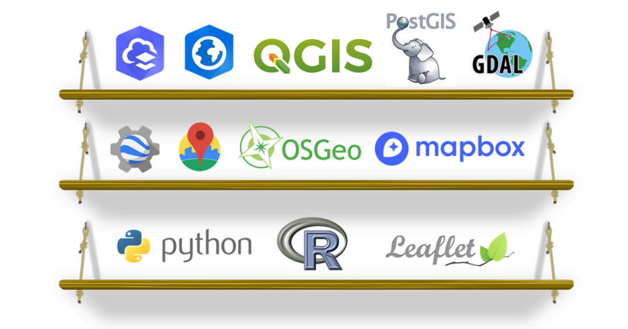
books, blog posts, videos,
online courses, tutorials, forums

Outline

Part 1

Integrating R and GIS
R’s spatial ecosystem
sf classes
Importing vector data
Managing projections
Subsetting features and attributes
Plotting with ggplot
Exercise 1

R - GIS Integration

GIS is no longer one thing!

Selecting Geospatial Software for a Project, IGIS Tech Note

‘Either-or’ is not the best way to to think about your options

A better question:

How to combine R with desktop and cloud GIS?

Roles that R can play

R as a replacement for (some) GIS tasks
especially where data is concerned
Automating workflows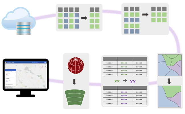

Preparing Reference GIS Layers for a Web Map with R
R for Spatial Analysis
example: Forest Tools
Accessing resources with R
API clients often come out fast and first in Open Source
R as a command and control center

Where R shines

Spatial stats
Reporting
Shiny apps
R as a development platform
Sharing code and data as packages
Out-of-the-box operations
new spatial and statistic techniques
Generating new data from scratch

Integrating R and GIS

R ↔︎ ArcGIS
R-ArcGIS Bridge
arcgislayers, arcgisgeocode, arcgisplaces, arcgisutils
R ↔︎ QGIS
Use R scripts in Processing plugin
R ↔︎ Cloud data and services
sf
gdalUtilities
httr2
API packages

R and Python

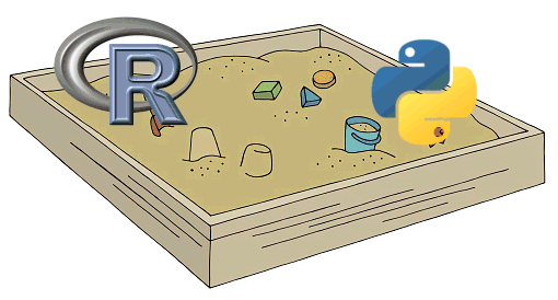
R and Python play very well together.

Where Python Shines

Integration with ArcGIS ecosystem
Latest Deep Learning models

R’s Spatial Ecosystem

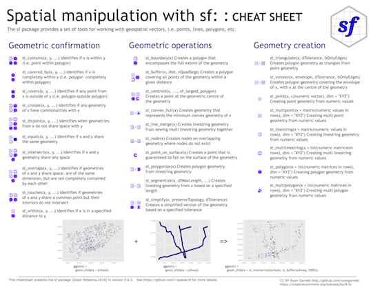
`sf`

sf is a popular package for working with vector geospatial data

sf stands for ‘simple feature’, which is a standard (developed by the Open Geospatial Consortium) for storing various geometry types in a hierarchical data model.

A ‘feature’ is just a representation of a thing in the real world (e.g. a building, a city, ).

Package features:

read / write / create / edit / manipulate GIS data in R
leverages open source libraries: GDAL, GEOS, PROJ
fast IO
enhanced plotting
objects are supported by an increasing number of other geospatial packages
aligns with other GIS software that use the sf data model (e.g. QGIS, PostGIS)

Simple Features

Simple features is an ISO standard for storing and accessing spatial data. It is widely adopted in spatial databases, open source formats like GeoJSON, GIS software, tools, etc.

Supports all standard geometry types:

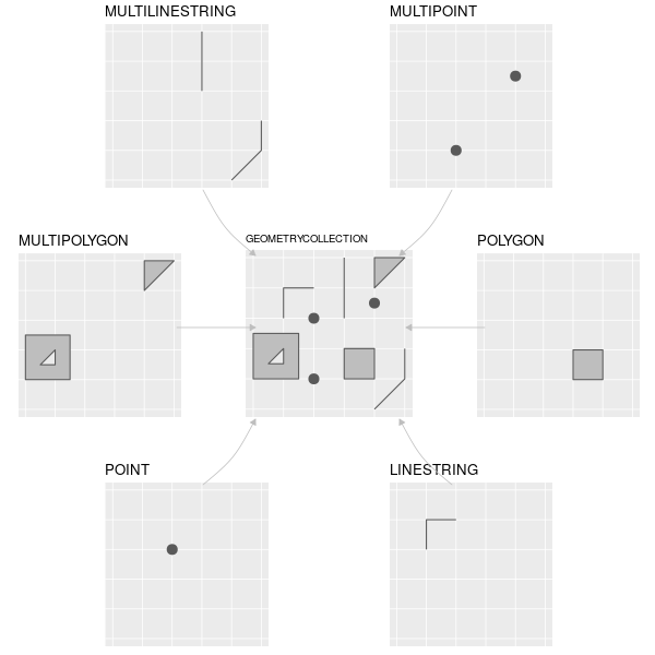
The geometry is encoded in a column using a standard called “Well Known Text” (WKT).

point	POINT (2 4)
multipoint	MULTIPOINT (2 2, 3 3, 3 2)
linestring	LINESTRING (0 3, 1 4, 2 3)
polygon	POLYGON ((1 0, 3 4, 5 1, 1 0))

sf object = date frame + 'geometry' column (WKT) + spatial metadata

sf example

library(sf)
nc <- st_read(system.file("shape/nc.shp", package="sf"), quiet = TRUE)
class(nc)

## [1] "sf"         "data.frame"

nc |> head()

## Simple feature collection with 6 features and 14 fields
## Geometry type: MULTIPOLYGON
## Dimension:     XY
## Bounding box:  xmin: -81.74107 ymin: 36.07282 xmax: -75.77316 ymax: 36.58965
## Geodetic CRS:  NAD27
##    AREA PERIMETER CNTY_ CNTY_ID        NAME  FIPS FIPSNO CRESS_ID BIR74 SID74
## 1 0.114     1.442  1825    1825        Ashe 37009  37009        5  1091     1
## 2 0.061     1.231  1827    1827   Alleghany 37005  37005        3   487     0
## 3 0.143     1.630  1828    1828       Surry 37171  37171       86  3188     5
## 4 0.070     2.968  1831    1831   Currituck 37053  37053       27   508     1
## 5 0.153     2.206  1832    1832 Northampton 37131  37131       66  1421     9
## 6 0.097     1.670  1833    1833    Hertford 37091  37091       46  1452     7
##   NWBIR74 BIR79 SID79 NWBIR79                       geometry
## 1      10  1364     0      19 MULTIPOLYGON (((-81.47276 3...
## 2      10   542     3      12 MULTIPOLYGON (((-81.23989 3...
## 3     208  3616     6     260 MULTIPOLYGON (((-80.45634 3...
## 4     123   830     2     145 MULTIPOLYGON (((-76.00897 3...
## 5    1066  1606     3    1197 MULTIPOLYGON (((-77.21767 3...
## 6     954  1838     5    1237 MULTIPOLYGON (((-76.74506 3...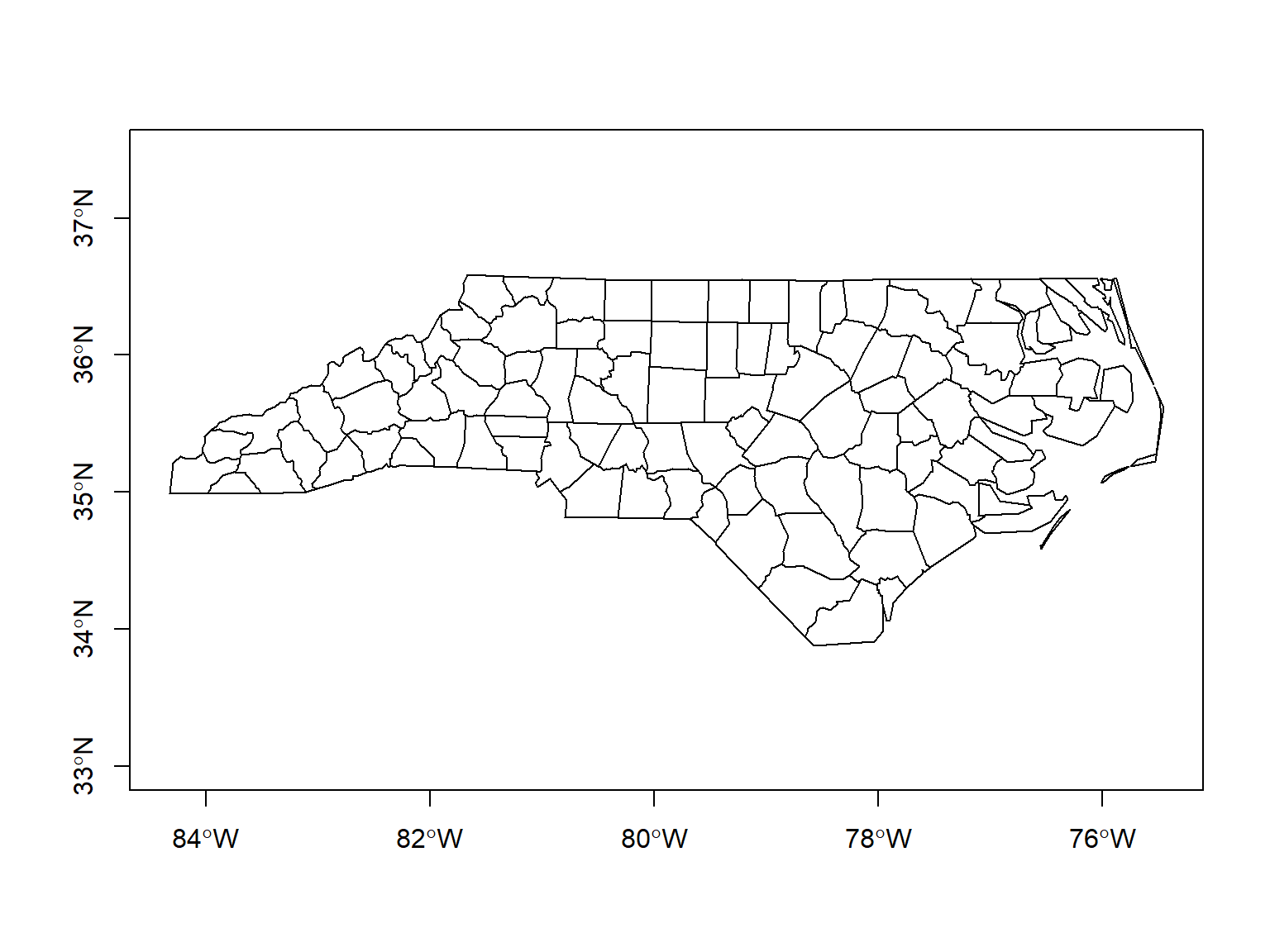

plot(nc$geometry, axes = TRUE)

`sf` functions

consistent function names (most start with st_)
|> pipe friendly!
everything you can do with a regular data frame, you can do with a sf data frame (almost)
integrated with the tidyverse packages

Importing Vector GIS Data with `sf`

To import GIS data with sf, you have to specify a source and potentially a layer.

The Source can be a:

folder: "./gis_data"

geodatabase (which is really a folder): "./gis_data/yose_roads.gdb"

file: "trail_heads.kml", "cell_towers.geojson"

database connection string: "PG:dbname=postgis"

The Layer can be a:

Shapefile name (minus the shp extension)

a named layer in the database / file

The two main functions for importing vector data are:

st_layers(source) - returns the names of available layers in a source

st_read(source, layer) - import into R

The argument for the source is dsn (data source name).

st_layers() also tells you the CRS and the number of rows & columns.

Projections

How do we squish a round planet onto flat maps / screens?

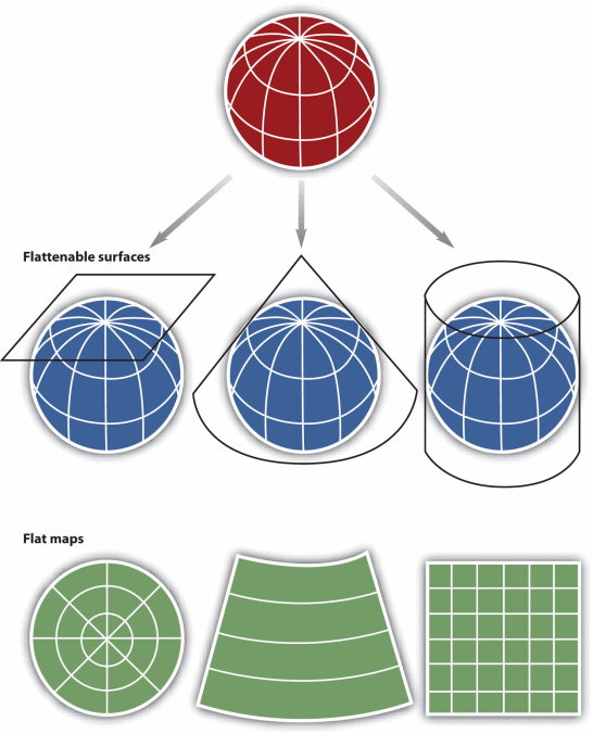
The more generic term for projections is ‘Coordinate Reference System’ (CRS).

CRS also includes ‘unprojected’ geographic coordinates (longitude & latitude).

There are 1,000s of CRS’s!

Each one has an EPSG number.

Why do I need to know this?

Projections are particularly important in R whenever you want to:

overlay layers in a plot (most R packages do not reproject on the fly)
compute or use geometric measurements, like distance or area
do spatial queries or joins

How `sf` handles CRS info

sf objects save CRS info

st_read() reads the CRS info when you import GIS data

st_write() writes the CRS info when you export GIS data

st_transform() (re)projects sf objects from one CRS to another

st_crs() views or assigns a CRS to a sf object

Common EPSG Numbers

Geographic CRSs

4326. Geographic, WGS84 (default for lon/lat)
4269. Geographic, NAD83 (USA Fed agencies like Census)

Projected CRSs

5070. USA Contiguous Albers Equal Area Conic
3310. CA Albers Equal Area
32610. UTM Zone 10, WGS84 (Northern Cal)
32611. UTM Zone 11, WGS84 (Southern Cal)
3857. Web Mercator (web maps)

The one-stop shop for finding EPSG numbers and PROJ4 strings is http://www.spatialreference.org. (Google usually works also).

Reference code for your convenience:

## Some common epsg numbers in California
epsg_geo_wgs84 <- 4326
epsg_geo_nad83 <- 4269
epsg_utm10n_wgs84 <- 32610
epsg_utm11n_wgs84 <- 32611
epsg_utm10n_nad83 <- 26910
epsg_utm11n_nad83 <- 26911
epsg_webmerc <- 3857
epsg_caalbers <- 3310

To view all EPSG codes (>5,500), run rgdal::make_EPSG()

`arcgislayers`

arcgislayers package (by Josiah Parry) provides an R interface to work with ArcGIS services on ArcGIS.com and ArcGIS Portal using the API

Key functions include:

importing vector and raster data from ArcGIS.com into R
publishing / updated data that you have created in R
performing raster functions (on the server)

This is really useful, because:

many government agencies publish GIS data with ArcGIS
if the data are publicly available, you don’t need an ArcGIS.com account to download it
you don’t need ArcGIS Pro
you can pass both attribute and spatial filters when requesting data (which will be executed on the server)

Import Data from ArcGIS.com - Workflow

Go to the “item details” page on ArcGIS.com for the layer you want.
Find the URL for the FeatureServer or MapServer.
Create a connection to the FeatureServer or MapServer (with arc_open()).
Use get_layer() to create a connection to the specific FeatureLayer you want to import.
Import the layer using arc_select(), providing an attribute and/or spatial query expression if needed.
The layer comes into R as a simple feature (sf) object

Example: Import Public Data from ArcGIS.com

library(sf)
library(arcgislayers)

## URL for a pubicly available Feature Server
counties_featsrv_url <- "https://services.arcgis.com/P3ePLMYs2RVChkJx/ArcGIS/rest/services/USA_Counties_Generalized_Boundaries/FeatureServer/"

## Create a FeatureServer object
counties_featsrv_fs <- arc_open(counties_featsrv_url)
counties_featsrv_fs

## <FeatureServer <1 layer, 0 tables>>
## CRS: 4326
## Capabilities: Query,Extract
##   0: USA Counties - Generalized (esriGeometryPolygon)

## List the layers available
arcgislayers::list_items(counties_featsrv_fs)

## # A data frame: 1 × 9
##      id name       parentLayerId defaultVisibility subLayerIds minScale maxScale
## * <int> <chr>              <int> <lgl>             <lgl>          <int>    <int>
## 1     0 USA Count…            -1 TRUE              NA                 0        0
## # ℹ 2 more variables: type <chr>, geometryType <chr>

## Create a FeatureLayer object
counties_featsrv_fl <- arcgislayers::get_layer(counties_featsrv_fs, id = 0)
counties_featsrv_fl

## <FeatureLayer>
## Name: USA Counties - Generalized
## Geometry Type: esriGeometryPolygon
## CRS: 4326
## Capabilities: Query,Extract

## View the fields in the attribute table
## list_fields(counties_featsrv_fl) |> View()

## Import just the Florida Counties
fl_counties_sf <- arc_select(counties_featsrv_fl, where = "STATE_FIPS = '12'")

plot(fl_counties_sf$geometry, axes = TRUE)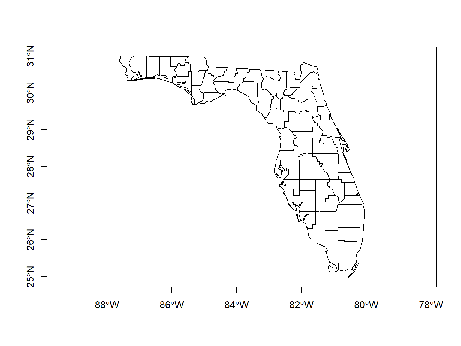

To import non-public data from ArcGIS online / portal, you need to authenticate by:

Create a Developer Auth Credentials (i.e., a service account) by logging into ArcGIS.com > Content > Add Content > New Developer Auth Credentials).
Feed your ‘client id’ and ‘client secret’ into arcgisutils::auth_code() or arcgisutils::auth_client() to generate a temporary token.
Pass the token to arc_open(), arc_select(), and other functions where needed.
Refresh the token when needed with arcgisutils::refresh_token().

ggplot

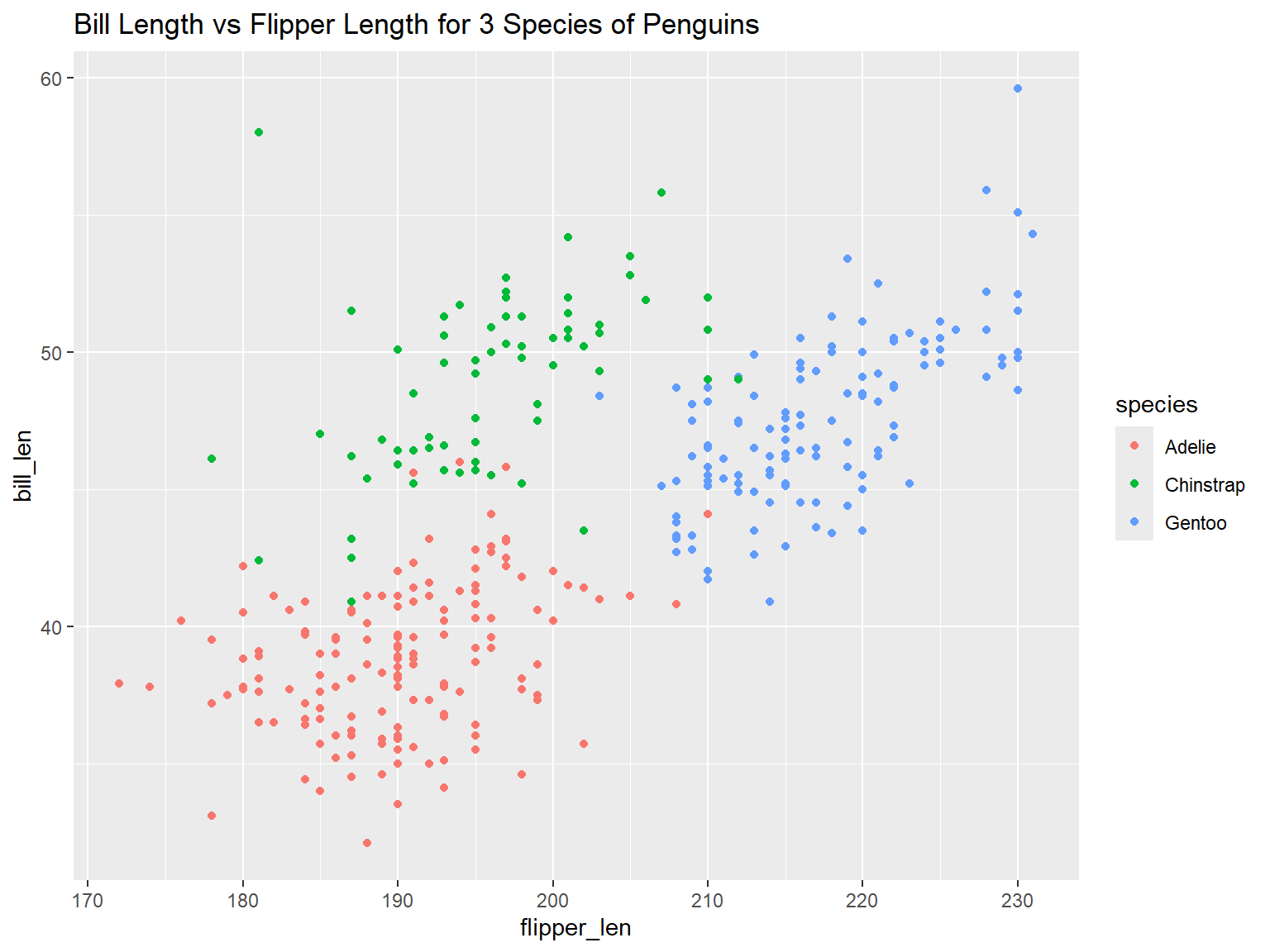
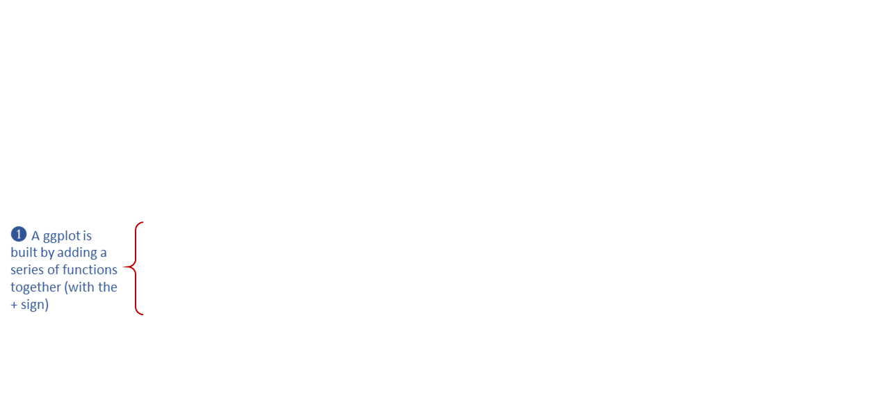
ggplots are constructed using the ‘grammar of graphics’ paradigm.

library(ggplot2)
ggplot(penguins, aes(x = flipper_len, y = bill_len, color = species)) +
  geom_point() +
  ggtitle("Bill Length vs Flipper Length for 3 Species of Penguins")

Anatomy of a ggplot

Maping Columns to Symbology with `aes()`

ggplot(penguins, aes(x = flipper_length_mm , y = bill_length_mm , color = species)) +
  geom_point() +
  ggtitle("Bill Length vs Flipper Length for 3 Species of Penguins")

aes() sets the default source for each visual property (or aesthetic) of the plot layers
- note you don’t need to put column names in quotes
some common visual properties:

x - where it falls along the x-axis
y - where it falls along the y-axis
color
fill
size
linewidth

which visual properties are needed depends on the geom_xxxx() functions you use
only put in aes() the visual properties you want linked to the data

Geoms

geom_xxxx() functions draw layers on the plot canvas
drawn from the bottom up
some common geoms:

geom_point()

geom_bar()

geom_boxplot()

geom_histogram()

visual properties can be linked to a column in the data frame or manually specified

geom_point(col = pop_size)

geom_point(col = “red”)

visual properties are inherited (from aes())
each geom has default color palettes and legend settings

Example

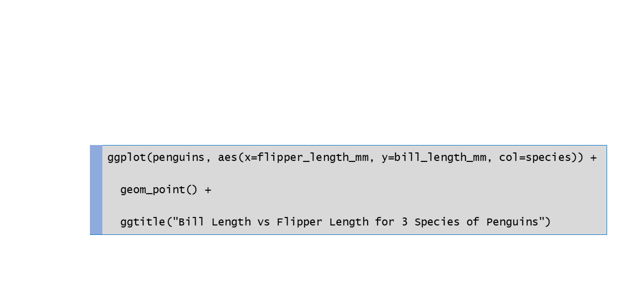
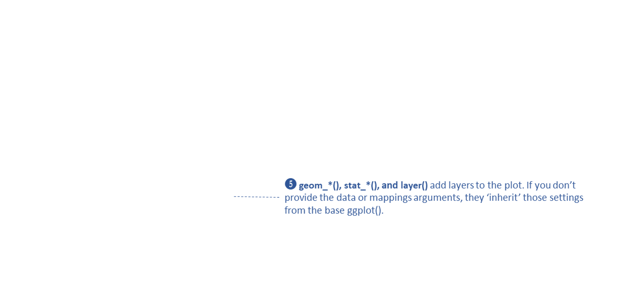
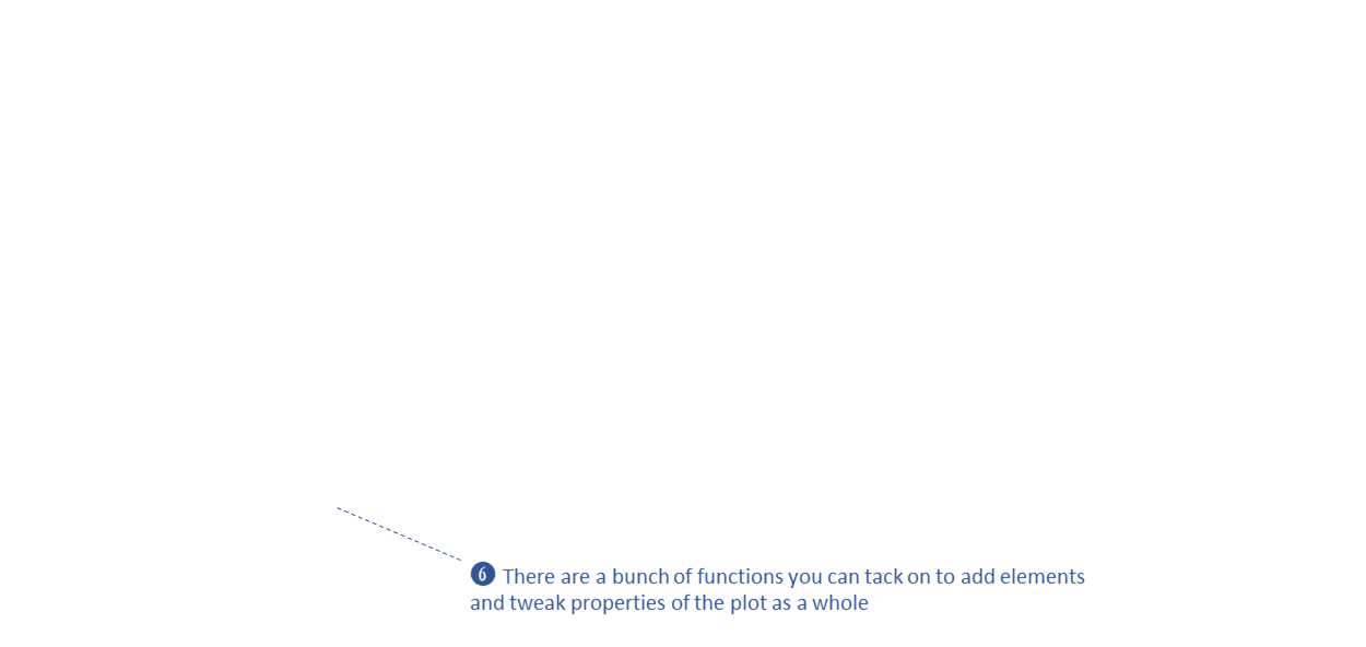
In the example below, note where geom_boxplot() gets its visual properties:

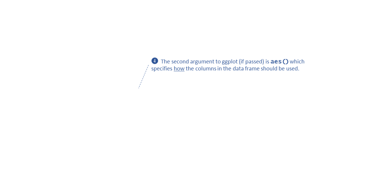
x and y are linked to columns in the dataframe and inherited from aes()
color, fill, and size are manually specified

ggplot(penguins, aes(x = species, y = bill_len)) +
  geom_boxplot(color = "navy", fill = "yellow", size = 1.5)

## Warning: Removed 2 rows containing non-finite outside the scale range
## (`stat_boxplot()`).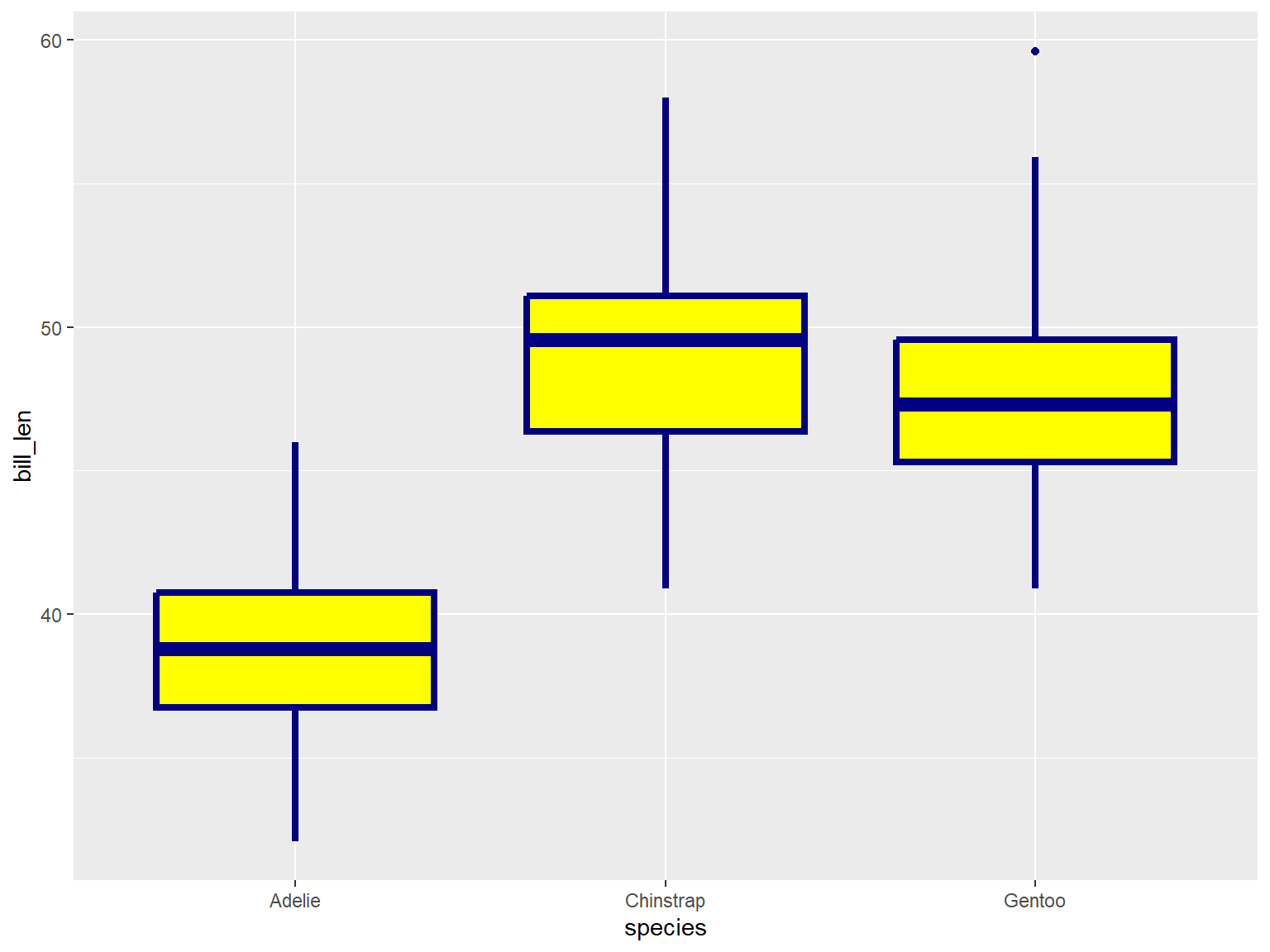

Mapping with ggplot

Making ggplots with geospatial data (i.e., maps) is not that different than regular ggplots.

A few differences:

we use sf objects as the data source (must all be in the same CRS)
draw layers with geom_sf()
most layers will be based on different spatial data, so in general there is no need to define data in the opening ggplot()
order of the layers matters
the ggspatial package has functions you can use to add other map elements (e.g., scale bar)

`geom_sf()`

The magical powers of geom_sf():

no need to define the columns for ‘x’ and ‘y’ in aes(), geom_sf() figures it out!
geom_sf() will draw points, lines or polygons, depending on the feature type
Just like other geom functions, geom_sf() provides lots of options to customize the visual properties. Most of these can be mapped to attribute fields!

fill: fill color
color: outline color
size: size of points, thickness of lines
shape: shape of points
linetype: line pattern

Example

library(sf)
library(ggplot2)

nc <- st_read(system.file("shape/nc.shp", package="sf"), quiet = TRUE)

ggplot() + 
  geom_sf(data = nc, aes(fill = BIR79)) +
  labs(title = "Live Births by County", 
       subtitle = "1979-1984")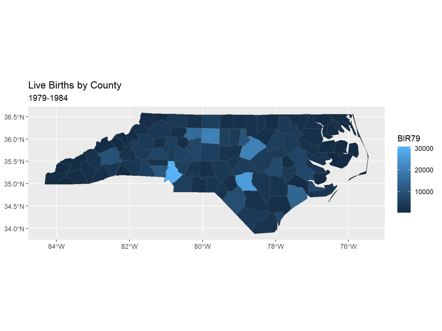

More info:
https://ggplot2-book.org/maps

Exercise 1

Break!

Repairing Geometries

Function	Fix
tidyr::drop_na(geometry)	drop rows where there geometry column contains NA
sf::st_zm()	Drop Z and/or M dimensions from feature geometries
sf::st_is_valid()	check if features have geometry problems
sf::st_make_valid()	repair common geometry problems

Spatial Data Fundamentals in R

Start Recording

About Me…

IGIS Team

Fall Workshops

Some of My R Work

R packages

Shiny Apps

About You

Workshop Goals

Leveraging Other Resources

Outline

Part 1

R - GIS Integration

GIS is no longer one thing!

‘Either-or’ is not the best way to to think about your options

A better question:

Roles that R can play

Where R shines

Integrating R and GIS

R and Python

Where Python Shines

R’s Spatial Ecosystem

sf

Simple Features

sf example

sf functions

Importing Vector GIS Data with sf

Projections

Why do I need to know this?

How sf handles CRS info

Common EPSG Numbers

Geographic CRSs

Projected CRSs

arcgislayers

Import Data from ArcGIS.com - Workflow

Example: Import Public Data from ArcGIS.com

ggplot

Anatomy of a ggplot

Maping Columns to Symbology with aes()

Geoms

Example

Mapping with ggplot

geom_sf()

Example

Exercise 1

Break!

Repairing Geometries

More Resources

`sf`

`sf` functions

Importing Vector GIS Data with `sf`

How `sf` handles CRS info

`arcgislayers`

Maping Columns to Symbology with `aes()`

`geom_sf()`