Computing Agroclimate Metrics in R
Part I. Intro and Simple Metrics
December
2,
2022
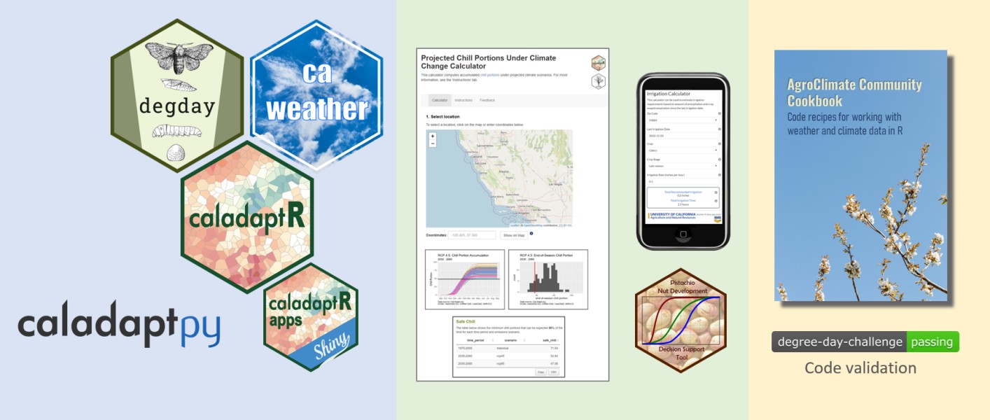
https://ucanr-igis.github.io/agroclimR/
![]()
December
2,
2022
https://ucanr-igis.github.io/agroclimR/
![]()

Type of Organization

Email domain

Location
Familiarity with Agroclimate Metrics

Familiarity with R

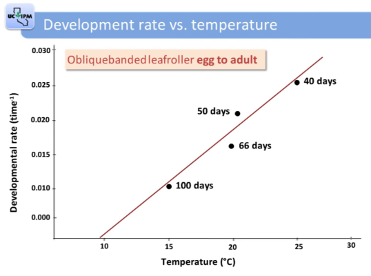
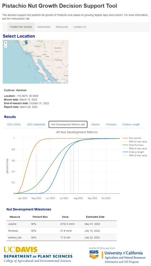
Pistachio nut embryo length vs
degree days
Zhang et al (2021)

 https://doi.org/10.1016/j.ufug.2018.07.020 |
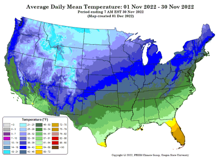
Where can I go today to see the climate my city will have 50 years from now? |
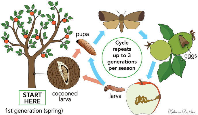
| How many generations of Navel Orangeworm will growers have to deal with in the coming decades? |
 https://doi.org/10.1016/j.scitotenv.2020.142657 |
 https://doi.org/doi:10.1371/journal.pone.0020155 |
How much chill can we expect in the coming decades? Will there be enough to have a economically viable farming operation? |
| What kind of frost exposure will we see mid-century? |
 https://doi.org/10.1016/j.scitotenv.2020.143971 |
 https://doi.org/10.3390/agronomy12010205 |
What is the ‘new normal’ for agroclimatic metrics for specialty crops? |
R is an extremely flexible computing environment,
with
strengths in:

![]()
![]()
![]()
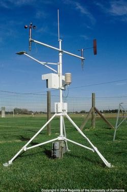
owmr:
OpenWeatherMap API Wrapper
rnoaa: ‘NOAA’
Weather Data from R
riem: Accesses
Weather Data from the Iowa Environment Mesonet
…plus many
others
Or write your own!

![]()
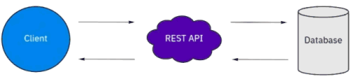
File server
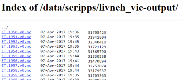
API service
Piping syntax is an alternative way of chaining functions together than nested parentheses:
zoo(moo(boo(foo(99),k=7),n=4))
With piping, you use the pipe operator |> or %>% to ‘feed’ the result of one function as the first argument to the next function.


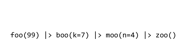
ctrl + shift + m|> (‘native’
pipe introduced R4.0)%>% (traditional, requires
magrittr package)
Whatever is needed to get your data frame ready for the
function(s)
you need for analysis and visualization.

The go-to package for wrangling data frames is dplyr:
![]()
dplyr Functions| subset rows | filter(), slice() |
| order rows | arrange(), arrange(desc()) |
| pick column(s) | select(), pull() |
| add new columns | mutate() |
| offset rows | lead(), lag() |
| vectorized conditional checks | if_else(), case_when() |
| join data frames | left_join(), right_join(), inner_join() |
Reshaping data includes:
The go-to tidyverse package for reshaping data frames is tidyr:
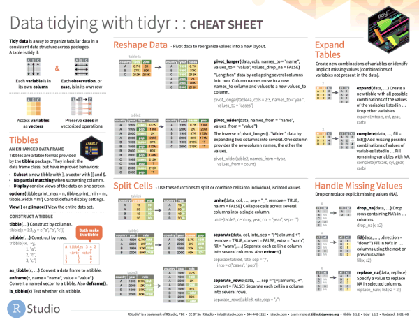
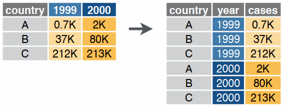
tidyr Functionspivot_wider()
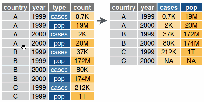
pivot_longer()
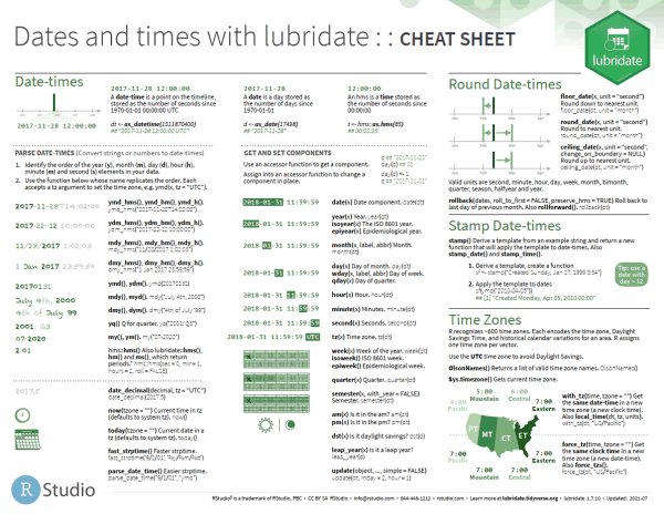
Agroclimate metrics frequently requires working with date values.
These are not Date objects:
x <- "2021-06-15"

y <- "4/1/2019"
To convert date-formatted text to Date objects use
as.Date():
bloom_date <- as.Date("2021-04-15")
class(bloom_date)
## [1] "Date"
For everything else…
rle()Heat spells or heat waves are often defined as number of consecutive days where the maximum temperature exceeds a certain threshold.
It is relatively easy to flag which days exceed a threshold:
grwsn_hotyn <- grwsn_dailymax_tbl |>
  mutate(hotyn = (max_temp > 100))
We can pull out consecutive days of high temperatures with the
rle() function.
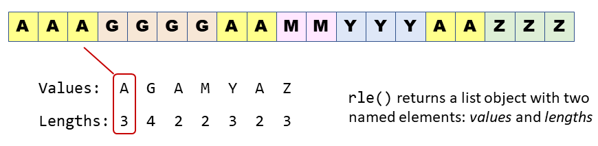
rle()Run length encoding is a way to compress data that is i) ordered, and ii) has repetitions. The best way to see how it works is with an illustration:
Now imagine we have time series data where TRUE means a hot day:
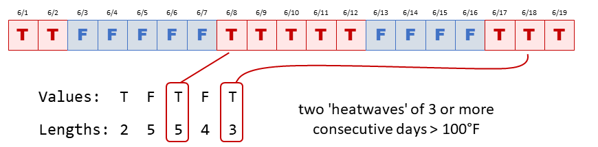
To compute this with rle():
hotdays_df <- data.frame(dt = seq(from = as.Date("2020-06-01"), to = as.Date("2020-06-19"), by = 1),
                      hotyn = c(T,T,F,F,F,F,F,T,T,T,T,T,F,F,F,F,T,T,T))
hotdays_df
## dt hotyn
## 1 2020-06-01 TRUE
## 2 2020-06-02 TRUE
## 3 2020-06-03 FALSE
## 4 2020-06-04 FALSE
## 5 2020-06-05 FALSE
## 6 2020-06-06 FALSE
## 7 2020-06-07 FALSE
## 8 2020-06-08 TRUE
## 9 2020-06-09 TRUE
## 10 2020-06-10 TRUE
## 11 2020-06-11 TRUE
## 12 2020-06-12 TRUE
## 13 2020-06-13 FALSE
## 14 2020-06-14 FALSE
## 15 2020-06-15 FALSE
## 16 2020-06-16 FALSE
## 17 2020-06-17 TRUE
## 18 2020-06-18 TRUE
## 19 2020-06-19 TRUE
First, run the vector in rle():
x <- rle(hotdays_df$hotyn)
x$values
## [1] TRUE FALSE TRUE FALSE TRUEx$lengths## [1] 2 5 5 4 3
Now we can write R expressions to pull out what we want.
## Which groups meet both conditions to be a heat wave?
group_is_heatwave <- (x$values == TRUE) & (x$lengths >= 3)
group_is_heatwave
## [1] FALSE FALSE TRUE FALSE TRUE## Number of heatwaves in this period
sum(group_is_heatwave)## [1] 2
library(palmerpenguins)
head(penguins)
## # A tibble: 6 × 8
## species island bill_length_mm bill_depth_mm flipper_l…¹ body_…² sex year
## <fct> <fct> <dbl> <dbl> <int> <int> <fct> <int>
## 1 Adelie Torgersen 39.1 18.7 181 3750 male 2007
## 2 Adelie Torgersen 39.5 17.4 186 3800 fema… 2007
## 3 Adelie Torgersen 40.3 18 195 3250 fema… 2007
## 4 Adelie Torgersen NA NA NA NA <NA> 2007
## 5 Adelie Torgersen 36.7 19.3 193 3450 fema… 2007
## 6 Adelie Torgersen 39.3 20.6 190 3650 male 2007
## # … with abbreviated variable names ¹flipper_length_mm, ²body_mass_g
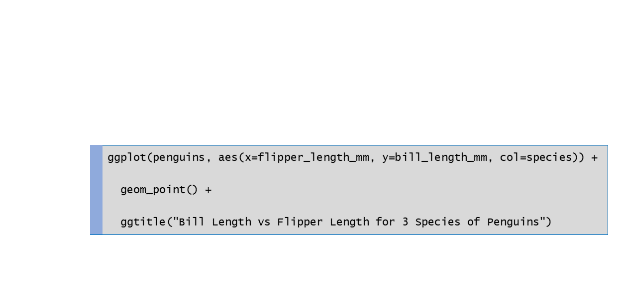
Make a scatter plot:
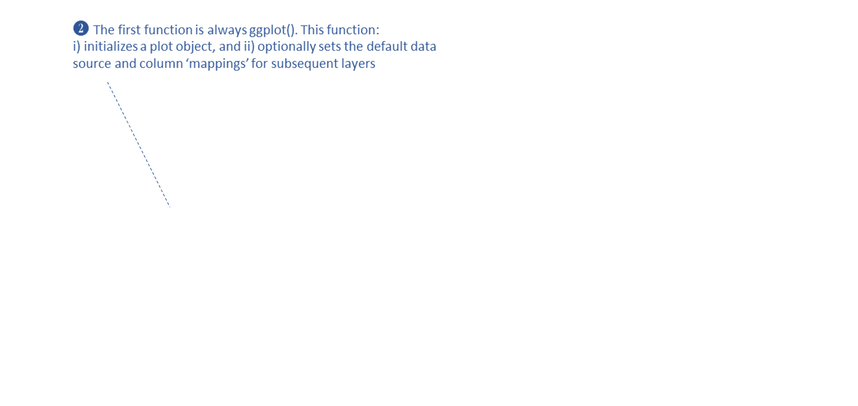
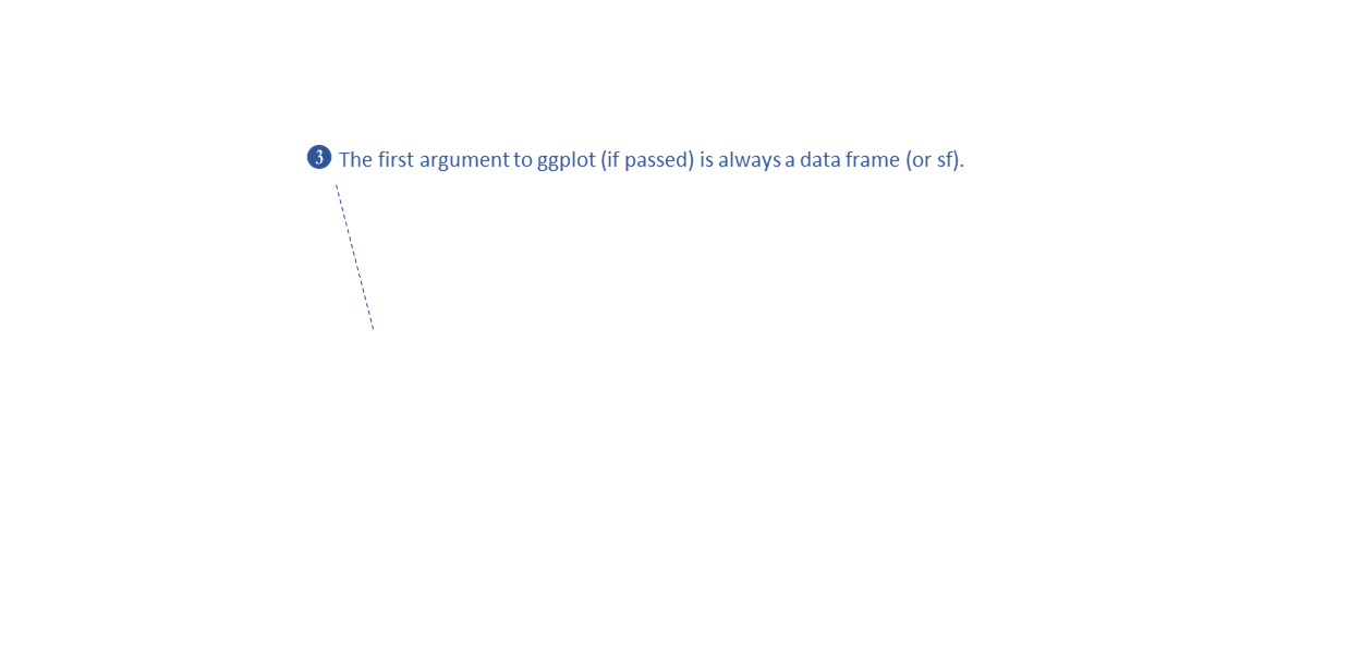
ggplot(penguins, aes(x = flipper_length_mm, y = bill_length_mm, color = species)) +
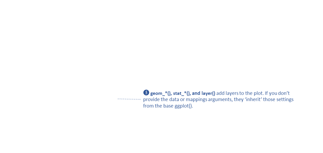
geom_point() +
ggtitle("Bill Length vs Flipper Length for 3 Species of Penguins")## Warning: Removed 2 rows containing missing values (`geom_point()`).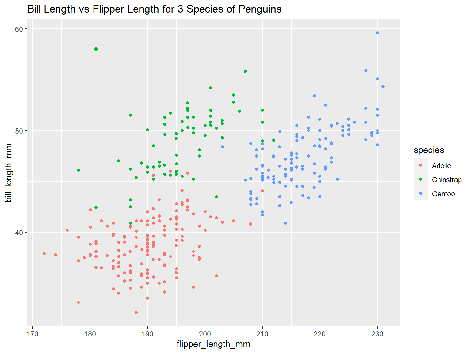


R Notebooks are written in “R Markdown”, which combines text and R code.
.png)
.png)
.png)
.png)
.png)
.png)
.png)
.png)
.png)
RStudio Cloud project for this workshop:
https://posit.cloud/content/5055980
After it opens:

Or see the Completed Notebook #1.