Computing Agroclimate Metrics in R
Part II. Cummulative Metrics and Multi-Year Summaries
December
2,
2022
https://ucanr-igis.github.io/agroclimR/
![]()
December
2,
2022
https://ucanr-igis.github.io/agroclimR/
![]()

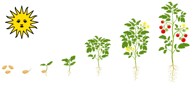
The timing of phenology events can be correlated with the sum amount of warmth within an organism’s usable range of temperature over a period of time
Researchers have explored several options:
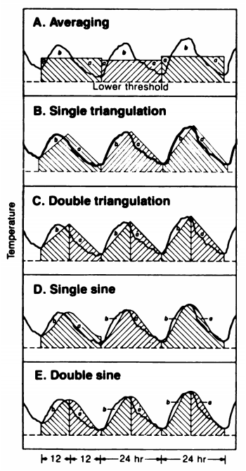
Zalom et al (1983)
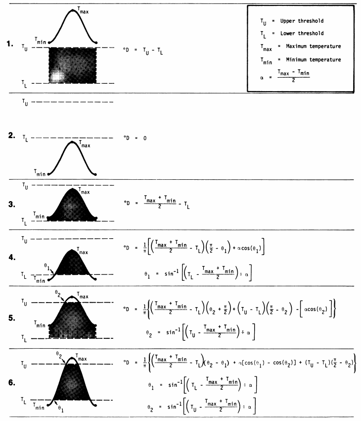
Zalom et al
(1983)


For a deeper dive into chill, see the e-book:
Tree Phenology Analysis with
R
by Eike Luedeling
For multi-year or multi-site data, you often need to work with groups of rows.
To work with groups in dplyr, we add functions that:
group_by()
The argument(s) to group_by() should be column(s) or
expression(s) that defines the row groups.
Each unique value will become a group of rows.
Example:
storms |>
  group_by(year) |>    ## group the rows by year
  head()
## # A tibble: 6 × 13
## # Groups: year [1]
## name year month day hour lat long status categ…¹ wind press…² tropi…³
## <chr> <dbl> <dbl> <int> <dbl> <dbl> <dbl> <chr> <ord> <int> <int> <int>
## 1 Amy 1975 6 27 0 27.5 -79 tropi… -1 25 1013 NA
## 2 Amy 1975 6 27 6 28.5 -79 tropi… -1 25 1013 NA
## 3 Amy 1975 6 27 12 29.5 -79 tropi… -1 25 1013 NA
## 4 Amy 1975 6 27 18 30.5 -79 tropi… -1 25 1013 NA
## 5 Amy 1975 6 28 0 31.5 -78.8 tropi… -1 25 1012 NA
## 6 Amy 1975 6 28 6 32.4 -78.7 tropi… -1 25 1012 NA
## # … with 1 more variable: hurricane_force_diameter <int>, and abbreviated
## # variable names ¹category, ²pressure, ³tropicalstorm_force_diameterNote - nothing looks different! This is because the groups are defined invisibly.
To do something productive with the groups, we have to add something else…
group_by() + mutate()
When working with cumulative metrics (i.e., chill portions) for
multiple years of data, you may want to calculate the metric for groups
of rows. You can compute metrics for groups of rows by following
group_by() with mutate().
Example:
We make a fake time series dataset consisting of a random number 0-10 each day for a year:
val_tbl <- tibble(dt = seq(from = as.Date("2010-01-01"),
                               to = as.Date("2010-06-30"),
                               by = 1)) |>
  mutate(val = runif(n(), min = 0, max = 10))

val_tbl |> head()
## # A tibble: 6 × 2
## dt val
## <date> <dbl>
## 1 2010-01-01 1.15
## 2 2010-01-02 4.58
## 3 2010-01-03 4.46
## 4 2010-01-04 5.44
## 5 2010-01-05 1.10
## 6 2010-01-06 6.11
Next we compute the cumulative sum of val for each month
(note how month is computed on-the-fly by
group_by()):
val_cumsum_bymonth_tbl <- val_tbl |>
  group_by(month = lubridate::month(dt)) |>
  mutate(cumsum_val = cumsum(val))

val_cumsum_bymonth_tbl |> head()
## # A tibble: 6 × 4
## # Groups: month [1]
## dt val month cumsum_val
## <date> <dbl> <dbl> <dbl>
## 1 2010-01-01 1.15 1 1.15
## 2 2010-01-02 4.58 1 5.73
## 3 2010-01-03 4.46 1 10.2
## 4 2010-01-04 5.44 1 15.6
## 5 2010-01-05 1.10 1 16.7
## 6 2010-01-06 6.11 1 22.8Plot it to see the pattern:
ggplot(val_cumsum_bymonth_tbl, aes(x = dt, y = cumsum_val)) + geom_line()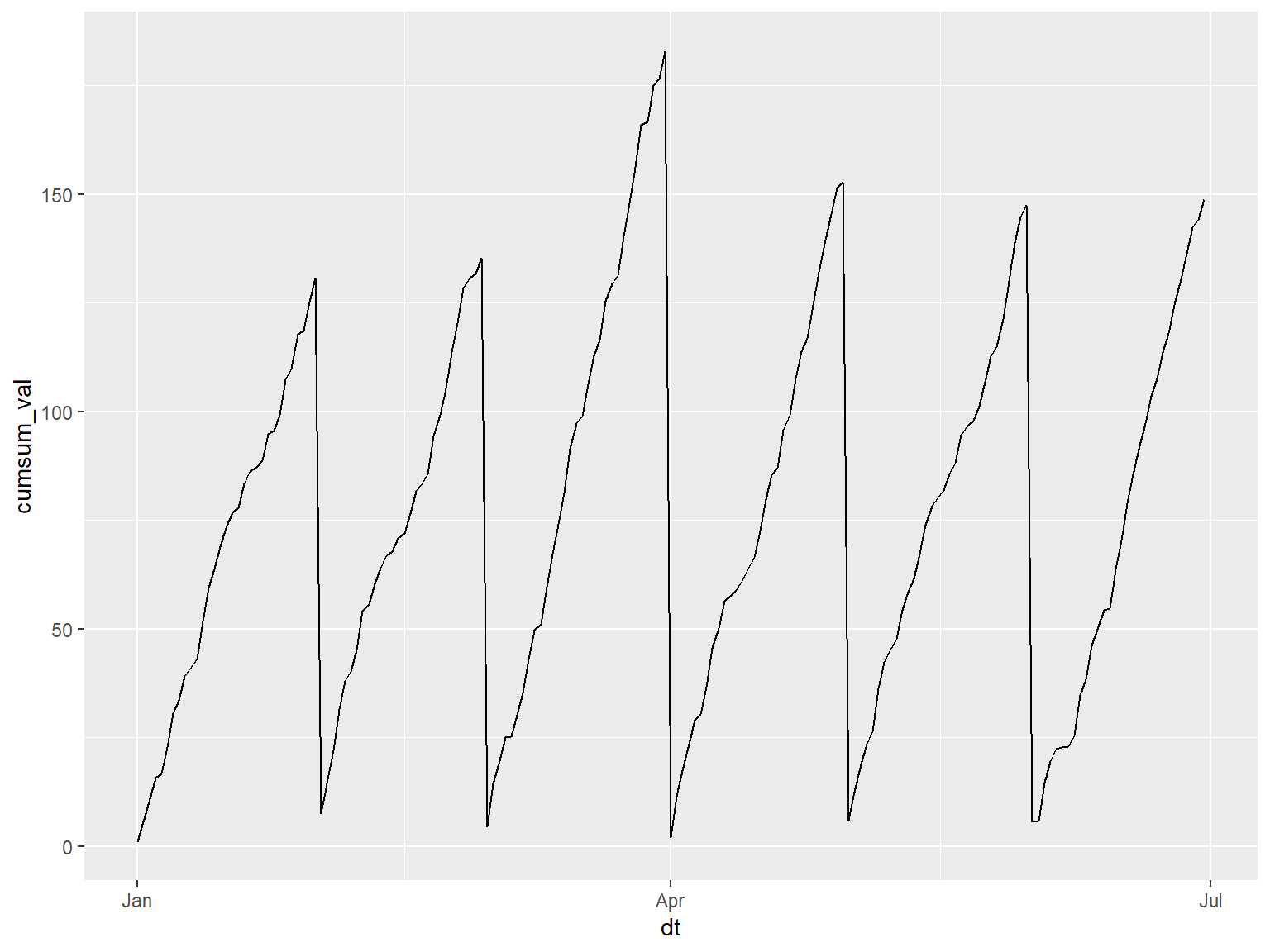
group_by() + summarize()
Commonly used in analysis,summarize() will create
column(s) of summary statistics for each group of rows.
To define the summaries, you can use any aggregate function that takes a vector of values and returns a single value. Examples:
n(), mean(), sum(), median(), min(), max(), first(), last(), sd(), IQR()
Example: How many category 4 and higher storms were there each month?
library(dplyr)

storms |>
  select(name, month, category, hurricane_force_diameter) |>         ## select the columns we need
  filter(category >= 4) |>                                           ## filter those rows where category >= 4
  group_by(month) |>                                                 ## group the rows by month
  summarize(num_hurricanes = n(),                                    ## for each group, report the count
            avg_diam = mean(hurricane_force_diameter, na.rm=TRUE))
## # A tibble: 5 × 3
## month num_hurricanes avg_diam
## <dbl> <int> <dbl>
## 1 7 12 63.6
## 2 8 95 92.9
## 3 9 275 86.7
## 4 10 91 78.2
## 5 11 24 51.9