Dissolve Boundaries Based on Attribute Fields

Grouping rows based on a common value of an attribute, and then computing one or more summary statistics for each group of rows, is extremely common. We a regular data frame, we can use group_by() and summarise() from dplyr.

We illustrate this with the attribute table from watersheds layer. This table has a column “HU” and “HUNAME” which are the id number and name of larger watersheds.

watersheds_df <- yose_watersheds %>% st_drop_geometry()
hu_df <- watersheds_df %>% 
  group_by(HU) %>% 
  summarise(HUNAME = first(HUNAME), 
            NUM_WATERSHEDS = n(),
            AVG_ACRES = mean(ACRES))
glimpse(hu_df)

## Rows: 6
## Columns: 4
## $ HU             <int> 1, 30, 31, 36, 37, 40
## $ HUNAME         <chr> "MONO", "EAST WALKER RIVER", "WEST WALKER RIVER", "TUOLUMNE RIVER", "MERCED RIVER", "SAN JOAQUIN RIVER"
## $ NUM_WATERSHEDS <int> 7, 5, 2, 60, 47, 6
## $ AVG_ACRES      <dbl> 9311.916, 9385.448, 6426.835, 8128.559, 8399.112, 8911.178

The exact same dplyr functions can be used with sf dataframes. The result is another sf object where the groups of features have been unioned together.

hu_sf <- yose_watersheds %>% 
  group_by(HU) %>% 
  summarise(HUNAME = first(HUNAME), 
            NUM_WATERSHEDS = n(),
            AVG_ACRES = mean(ACRES))
hu_sf

## Plot
tm_shape(hu_sf) + 
  tm_polygons(col="HUNAME", title="HU Watershed") + 
tm_shape(yose_watersheds) +
  tm_borders(col="gray60", lwd=0.8) +
tm_layout(legend.outside = T)

## Simple feature collection with 6 features and 4 fields
## Geometry type: POLYGON
## Dimension:     XY
## Bounding box:  xmin: 1383.82 ymin: -61442.93 xmax: 81596.71 ymax: 26405.66
## Projected CRS: unnamed
## # A tibble: 6 x 5
##      HU HUNAME            NUM_WATERSHEDS AVG_ACRES                                                                                         geom
##   <int> <chr>                      <int>     <dbl>                                                                                <POLYGON [m]>
## 1     1 MONO                           7     9312. ((70287.08 -14275.14, 70251.27 -14189.88, 70232.39 -14119.7, 70208.96 -14049.36, 70184.34...
## 2    30 EAST WALKER RIVER              5     9385. ((46352.24 12533.19, 46298.25 12538.45, 46213.04 12558.25, 46149.84 12579.34, 46028.1 126...
## 3    31 WEST WALKER RIVER              2     6427. ((37864.42 15722.13, 37835.53 15728.08, 37757.89 15760.15, 37722.95 15765.8, 37700.88 157...
## 4    36 TUOLUMNE RIVER                60     8129. ((3616.133 -14692.77, 3546.085 -14672.49, 3480.853 -14635.53, 3389.411 -14589.89, 3237.72...
## 5    37 MERCED RIVER                  47     8399. ((8262.059 -34088.83, 8205.085 -34130.97, 8164.326 -34131.78, 8067.706 -34151.91, 7969.99...
## 6    40 SAN JOAQUIN RIVER              6     8911. ((61771.61 -47929.25, 61796.63 -48002.35, 61803.31 -48129.88, 61801.05 -48214.62, 61807.2...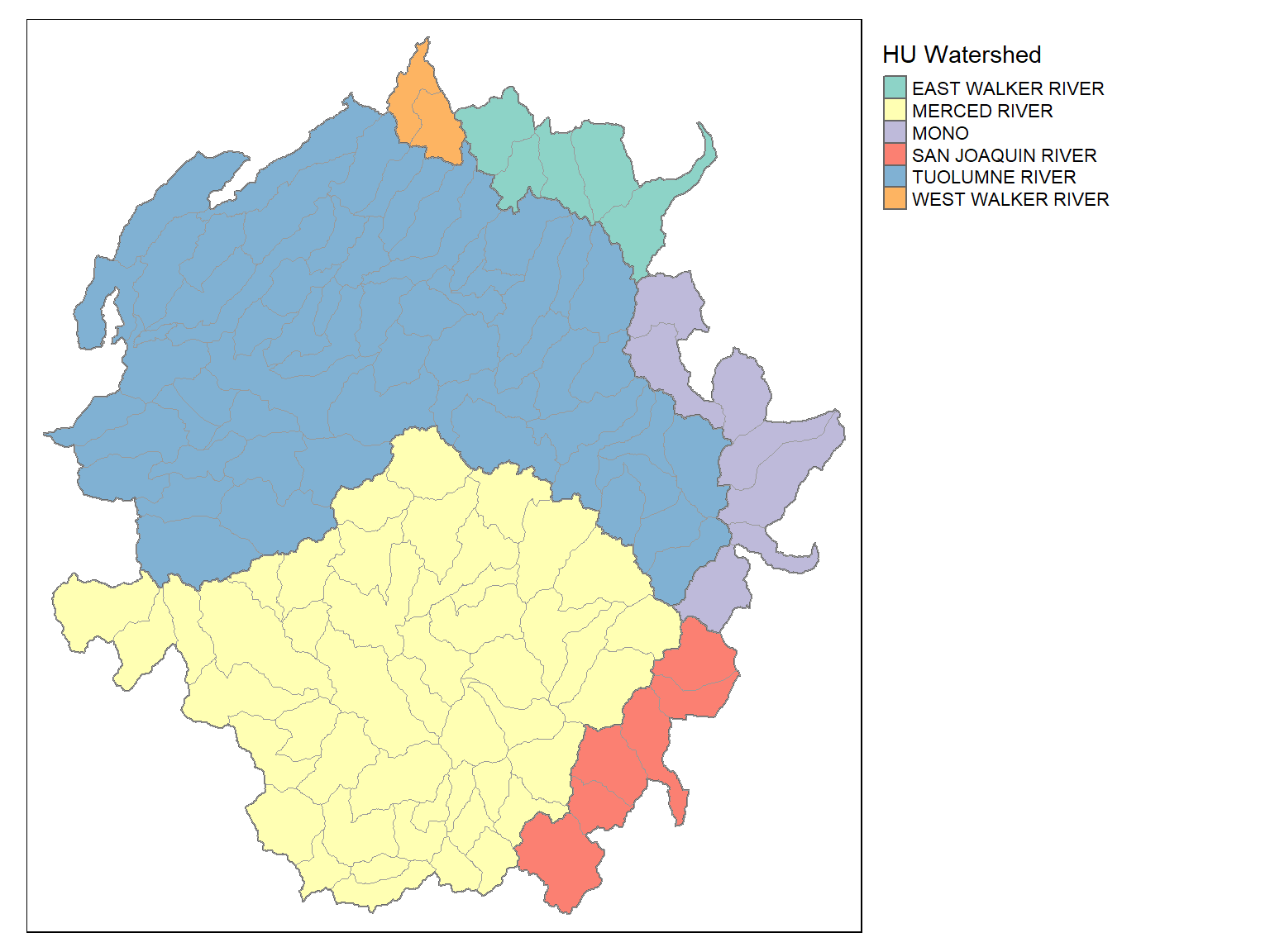

Geoprocessing Chains

What percentage of Yosemite falls within 500m of a road?

We first create a 500m buffer around the roads within the park (representing a disturbance zone for sensitive species, or drive transect detection area). Then we’ll compute the total area of the buffered area. This task will require us to buffer, intersect, union, and another intersection. This is known as a geoprocessing chain. . First, create the buffer:

## Create the buffer
yose_roads_buff <- yose_roads %>% st_buffer(dist=500)

## Plot the results
tm_shape(yose_roads_buff) + tm_polygons(col="red") +
tm_shape(yose_bnd_utm) + tm_borders(lwd=2)

There are two problems here:

1. the roads extend outside the park
2. the buffered line segments overlap each other (so we can’t add up the areas)

We can fix these by taking the intersection of the road buffer with the park boundary, and unioning the individual polygons together.

## Clip to park boundary
yose_roads_inpark_buff <- yose_roads_buff %>%
  st_intersection(yose_bnd_utm) %>% 
  st_union()

## Plot the results
tm_shape(yose_bnd_utm) + 
  tm_borders(lwd=2) +
tm_shape(yose_roads_inpark_buff) +
  tm_polygons(col="red")

What is the total area of the buffer?

road_area <- yose_roads_inpark_buff %>% 
  st_area() %>% 
  sum()
road_area %>% set_units(ha)

## 23879.94 [ha]

road_area / (yose_bnd_utm %>% st_area())

## 0.07907479 [1]

Voronoi Tesselation

For a given a set of points, Voronoi tesselation computes a network of polygons, such that each polygon contains exactly one point and everywhere within a polygon is closest to the enclosed point.

Let’s build Voronoi polygons for the campgrounds. These polygons could be thought of as the ‘catchment area’ of each campgrounds, if campgrounds were like magnets trying to attract campers.

We can create a Voronoi tessellation using st_voronoi(). Note st_voronoi() expects a single multipart point feature, which you can create from a point layer using st_union().

## Compute Voronoi polygons
v <- st_voronoi(st_union(yose_campgrnds_utm))

## Construct polygon sf and simplify (i.e., break multipart into single features)
v_sf <-  st_sf(v) %>% st_cast()

## Plot
plot(v_sf %>% st_geometry() , col = NA, border="gray70")
plot(yose_bnd_utm %>% st_geometry(), add=TRUE, col=NA, border="darkblue")
plot(yose_campgrnds_utm %>% st_geometry(), col="darkgreen", cex=1, pch=17, add=T)

## Clip to the park boundary
v_clipped <- v_sf %>% st_intersection(yose_bnd_utm)

plot(v_clipped %>% st_geometry() , col = NA, border="gray70")
plot(yose_bnd_utm %>% st_geometry(), add=TRUE, col=NA, border="darkblue")
plot(yose_campgrnds_utm %>% st_geometry(), col="darkgreen", cex=1, pch=17, add=T)

Summary

In this session we saw how to: