Spatial Queries

Spatial query = selecting features based on their location or spatial relationship (relative to another feature)

Spatial Querying is also known as Spatial Subsetting

Spatial relationship functions in sf:

st_intersects()	overlaps or touches
st_disjoint()	opposite of intersect
st_touches()	touches only
st_crosses()	cross (but doesn’t touch)
st_within()	within
st_contains()	contains
st_contains_properly()	interiors intersect but not edges or exterior
st_overlaps()	overlaps
st_equals()	equals
st_covers()	covers
st_covered_by()	completely covered
st_equals_exact()	equals within a tolerance
st_is_within_distance()	within a distance

These functions are also known as spatial predicates.

These are logical functions - they return TRUE/FALSE values (and/or or row numbers).

Spatial proximity functions require that layers be in the same CRS.

Using Logical Spatial Relationship Functions

Let’s look at an example:

st_intersects(x, y, sparse=TRUE)

where

x (target) and y (source) are both sf objects

sparse = TRUE

function returns a list object with
one element for each feature of x, and
each element contains the indices of y where the test is TRUE

sparse = FALSE

function returns a matrix of logical values, with
one row for each feature of x, and
one column for each features in y

Example: Points and Polygons

Consider an example where x contains 5 points and y contains 2 polygons:

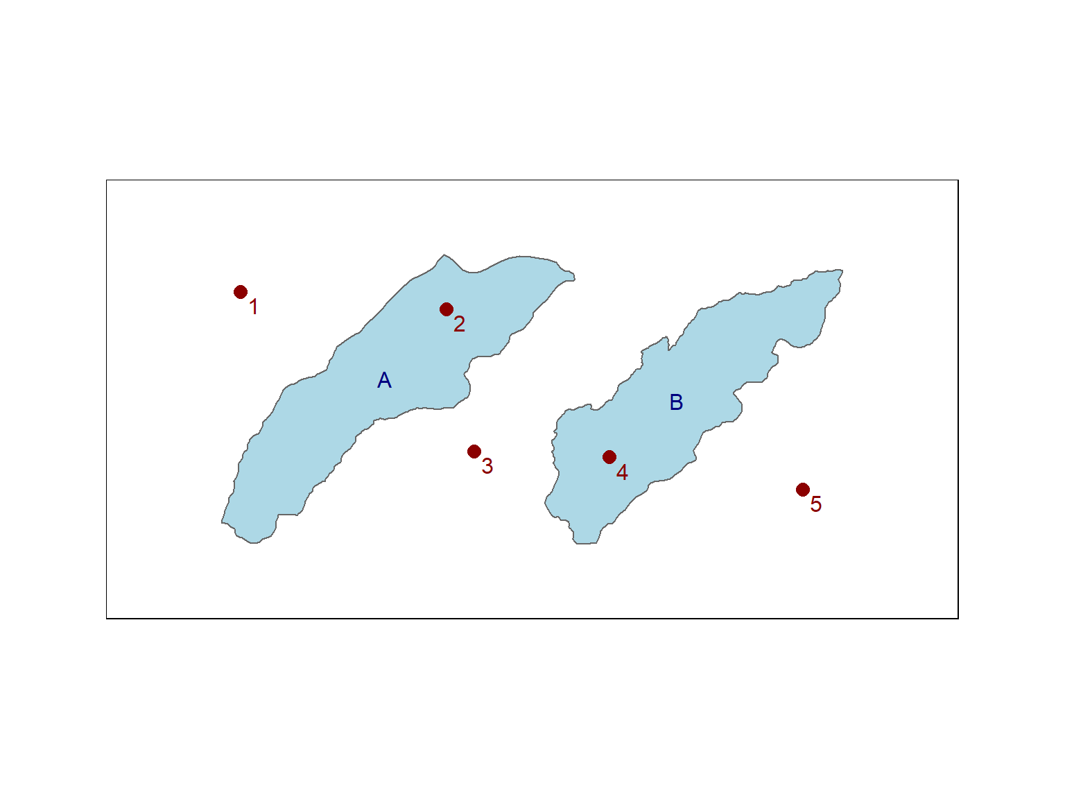
When sparse = TRUE, you get a list of indices:

st_intersects(my_pts, my_polys, sparse = TRUE)

## Sparse geometry binary predicate list of length 5, where the predicate was `intersects'
##  1: (empty)
##  2: 1
##  3: (empty)
##  4: 2
##  5: (empty)

When sparse = FALSE, you get a 2 x 5 matrix of logical values:

st_intersects(my_pts, my_polys, sparse = FALSE)

##       [,1]  [,2]
## [1,] FALSE FALSE
## [2,]  TRUE FALSE
## [3,] FALSE FALSE
## [4,] FALSE  TRUE
## [5,] FALSE FALSE

When you get back the results of a spatial relationship test, you can use them to subset features with dplyr functions:

feed TRUE / FALSE values into filter()
feed row numbers into slice()

R Notebook 1: Find Yosemite POIs that Intersect the Merced Watershed

nb_spatqry_01_scgis21.Rmd

Identify points-of-interest that fall within the Merced River watershed

preview notebook | answer key

Spatial Selection with Square Bracket Notation

You can also subset spatially use the familiar square bracket notation, putting a sf object as the expression for the rows.

The following are equivalent:

poi_merced2 <- yose_poi %>% st_intersection(merced_hu_utm)

poi_merced1 <- yose_poi[merced_hu_utm, ]

By default, when the rows argument is a sf object the result will be an intersection. To use a different spatial test, add the optional op argument:

## The following will return all features in yose_poi *except* where they intersect

## Note the blank space where the 'columns' expression should normally go.
## You still need that comma!

poi_not_merced <- yose_poi[merced_hu_utm, , op = st_disjoint]

Computing Distances

sf::st_distance() computes distances between pairs of features

If you pass it one sf object, it’ll return a distance matrix of features in that layer.

If you pass it two sf objects, it’ll return a pairwise distance matrix of features in both layer.

Example 1: Compute distances between cell towers

epsg_utm11n_nad83 <- 26911

yose_celltwrs_utm <- st_read("./data/yose_communications.gdb", "Cell_Towers", quiet = TRUE) %>% 
  st_transform(epsg_utm11n_nad83) %>% 
  select(tower_id = Id, tower_name = Name, x_utm = X_UTM, y_utm = Y_UTM)

st_distance(yose_celltwrs_utm) %>% round()

## Units: [m]
##       [,1]  [,2]  [,3]  [,4]  [,5]
## [1,]     0 25216 26523 45311 43318
## [2,] 25216     0  1892 22540 21140
## [3,] 26523  1892     0 20686 21215
## [4,] 45311 22540 20686     0 27738
## [5,] 43318 21140 21215 27738     0

distance is always computed in map units (so use projected data!)

st_distance() returns distances using the units package

Example 2: Compute distances between cell towers and campgrounds

## Import the campgrounds
yose_campgrnds_utm <- st_read(dsn="./data", layer="yose_poi", quiet = TRUE) %>% 
  filter(POITYPE == 'Campground') %>% 
  select(POINAME) %>% 
  st_transform(epsg_utm11n_nad83)

st_distance(yose_campgrnds_utm, yose_celltwrs_utm) %>% round()

## Units: [m]
##        [,1]  [,2]  [,3]  [,4]  [,5]
##  [1,] 46219 25885 26226 33538  5904
##  [2,] 42064 19211 19163 25492  2385
##  [3,] 36624 13645 13738 23774  7499
##  [4,] 26168 15613 17308 36062 19627
##  [5,] 22083  9689 11543 31666 21313
##  [6,] 20396  7834  9724 30322 22987
##  [7,]   541 24683 25995 44831 42783
##  [8,] 33353  9178  7376 13417 20586
##  [9,] 46362 23071 21252  1825 26769
## [10,] 26671  1890  2647 22221 19250
## [11,] 23859  1411  2822 23428 22413
## [12,] 23970  1403  2639 23199 22497
## [13,] 24176  1257  2426 22996 22384
## [14,] 24211  1734  2314 22612 22844
## [15,] 33272 26623 28245 45779 23754

Each row represents a campground.

Each column represents a cell tower.

Nearest Neighbors

To identify nearby neighbors, you can use:

st_is_within_distance() ()

st_nearest_feature()

st_nearest_points()

nngeo::st_nn()

Some of these return indices. Some of them return indices or logicals, some of them return geometries. See the help pages for details.

When computing feature-to-feature distances or identifying nearest neighbors, the layers should be in the same CRS.

Example: Find the closest trail to each campground

Here we’ll find the closest trail segment for each campground using st_nn() from the nngeo package.

## Import the trails
yose_trails_utm <- st_read("./data/yose_trails.gdb", layer="Trails") %>% 
  st_transform(epsg_utm11n_nad83)

## Load the nngeo package
library(nngeo)

## Run st_nn() passing sparse = TRUE so we get back a list of indices
closest_trail_lst <- st_nn(yose_campgrnds_utm, yose_trails_utm, sparse = TRUE, progress = FALSE)
glimpse(closest_trail_lst)

## Convert the list to a vector
closest_trail_idx <- unlist(closest_trail_lst)
closest_trail_idx

## Reading layer `Trails' from data source `D:\Workshops\R-Spatial\rspatial_mod\outputs\rspatial_data\data\yose_trails.gdb' using driver `OpenFileGDB'
## Simple feature collection with 1074 features and 13 fields
## Geometry type: MULTILINESTRING
## Dimension:     XY
## Bounding box:  xmin: 245134 ymin: 4153668 xmax: 323239.7 ymax: 4250703
## Projected CRS: NAD83 / UTM zone 11N
## List of 15
##  $ : int 610
##  $ : int 117
##  $ : int 275
##  $ : int 467
##  $ : int 504
##  $ : int 961
##  $ : int 237
##  $ : int 432
##  $ : int 343
##  $ : int 563
##  $ : int 541
##  $ : int 603
##  $ : int 566
##  $ : int 927
##  $ : int 72
##  [1] 610 117 275 467 504 961 237 432 343 563 541 603 566 927  72

Plot the results:

## Plot results
rainbow_cols <- rainbow(nrow(yose_campgrnds_utm), end=5/6)
tm_shape(yose_trails_utm, bbox=yose_campgrnds_utm) + 
  tm_lines(col="gray90") +
  tm_shape(yose_trails_utm %>% slice(closest_trail_idx)) + 
  tm_lines(col="red", lwd=2) +
  tm_shape(yose_campgrnds_utm) + 
  tm_symbols(col="POINAME", palette = rainbow_cols, size=0.5) + 
  tm_layout(legend.show = FALSE)

For large datasets or if you need more options, see also FNN (Fast Nearest Neighbor) package.

Spatial Joins

A spatial join is a lot like dplyr::left_join()

⇒ you’re copying attribute columns from one table to another.

But instead of joining two rows based on the values in a common column, you join them based on their spatial relationship.

In R you can do a spatial join with:

st_join(x, y, join)

where x and y are sf objects

join is the name of a spatial relationship function:

st_intersects
st_nearest_feature
st_is_within_distance
st_within
see ?st_join for others

ESRI calls spatial joins geo-enrichment

Example: For each campground, join attributes from the nearest cell tower

Use a spatial join to save the id and coordinates of the closest cell tower to the campgrounds attribute table.

yose_camp_plus_cell_utm <- yose_campgrnds_utm %>% 
  st_join(yose_celltwrs_utm, join = st_nearest_feature)

yose_camp_plus_cell_utm

## Simple feature collection with 15 features and 5 fields
## Geometry type: POINT
## Dimension:     XY
## Bounding box:  xmin: 247625.8 ymin: 4158885 xmax: 292815.1 ymax: 4204389
## Projected CRS: NAD83 / UTM zone 11N
## First 10 features:
##                        POINAME tower_id              tower_name    x_utm   y_utm
## 1    Hodgdon Meadow Campground       30              Crane Flat 251532.4 4182870
## 2        Crane Flat Campground       30              Crane Flat 251532.4 4182870
## 3     Tamarack Flat Campground       30              Crane Flat 251532.4 4182870
## 4        White Wolf Campground        6         Yosemite Valley 272489.8 4180099
## 5    Yosemite Creek Campground        6         Yosemite Valley 272489.8 4180099
## 6    Porcupine Flat Campground        6         Yosemite Valley 272489.8 4180099
## 7  Tuolumne Meadows Campground        3 Tuolumne Meadows (CDWR) 293307.2 4194328
## 8  Bridalveil Creek Campground       21           Sentinel Dome 272232.6 4178225
## 9            Wawona Campground       27                  Wawona 265240.0 4158756
## 10           Camp 4 Campground        6         Yosemite Valley 272489.8 4180099
##                    geometry
## 1  POINT (247625.8 4187296)
## 2  POINT (253315.9 4181287)
## 3  POINT (258936.4 4181679)
## 4  POINT (267142.6 4194768)
## 5  POINT (271702.9 4189756)
## 6  POINT (273987.5 4187789)
## 7  POINT (292815.1 4194103)
## 8  POINT (268815.7 4171688)
## 9  POINT (263419.9 4158885)
## 10   POINT (270612 4180317)

To extract values from a raster at feature locations, use raster::extract().

More Practice

nb_spatqry_02_scgis21.Rmd

Generate an exact number of sample points within YNP (random points plus spatial query); get the vegetation value at each sample location (spatial join); identify sample points within 2km of each campground (spatial query)

preview notebook | answer key

Summary

In this session we saw how to:

use functions like st_intersects() and st_is_within_distance() that test pairs of features for spatial relationships
use the results of spatial relationship functions to select features
compute distances between features
find the nearest feature(s) with st_nn()
do spatial joins

Additional Resources

Geocomputation with R Ch4: Spatial Data Operations. Robin Lovelace, Jakub Nowosad, Jannes Muenchow

Next: Raster Manipulations

Spatial Data Analysis with R Society for Conservation GIS, July 2021

Spatial Queries

Using Logical Spatial Relationship Functions

Example: Points and Polygons

R Notebook 1: Find Yosemite POIs that Intersect the Merced Watershed

Spatial Selection with Square Bracket Notation

Computing Distances

Example 1: Compute distances between cell towers

Example 2: Compute distances between cell towers and campgrounds

Nearest Neighbors

Example: Find the closest trail to each campground

Spatial Joins

Example: For each campground, join attributes from the nearest cell tower

More Practice

Summary

Spatial Data Analysis with R
Society for Conservation GIS, July 2021