Chapter 8 Raster Operations

Downloading Cal-Adapt climate data as rasters makes sense if your analysis involves methods that require the entire surface, and/or uses raster methods such as delineating isopleths, classification, or stacking on other raster layers. You may also want to use rasters simply for convenience, for example if you have a lot of sample points and/or will be extracting values many times. Downloading rasters only has to be done once, after which you can query them locally.

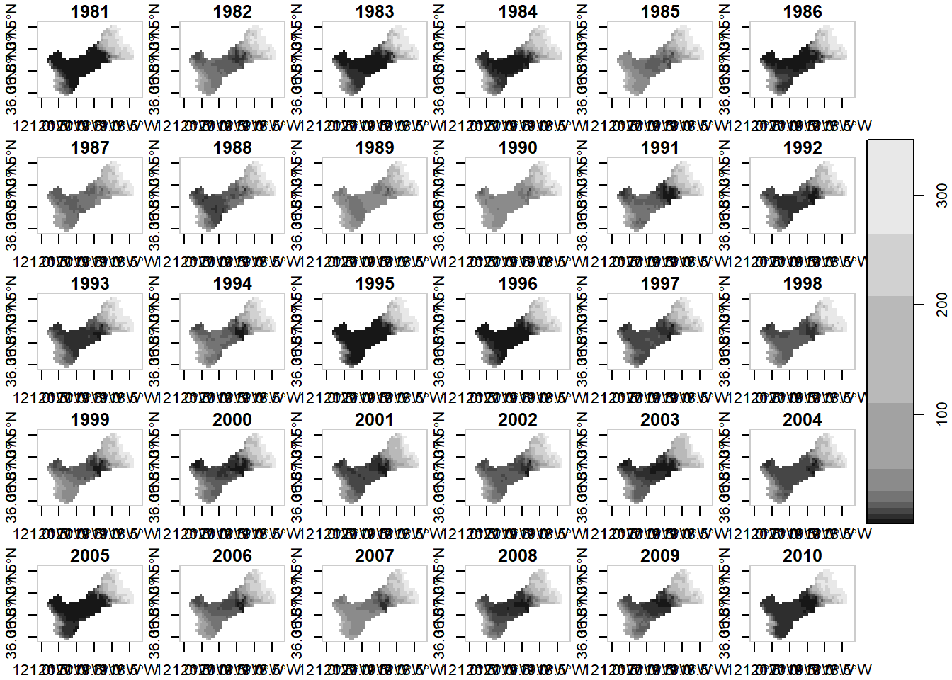
In this chapter, we’ll see how to download rasters to compute the number of frost days across Fresno county, which is a large county that includes both valley and mountainous areas. Our first output will be a raster that shows the number of frost days per year for 30 years of observed minimum daily temperature.

8.1 Load Packages

As usual, we start by loading a bunch of packages into memory and specifying our preferences for conflicting function names:

library(caladaptr)
library(units)
library(ggplot2)
library(dplyr)
library(tidyr)
library(lubridate)
library(sf)
library(stars)

Set conflicted preferences:

library(conflicted)
conflict_prefer("filter", "dplyr", quiet = TRUE)
conflict_prefer("count", "dplyr", quiet = TRUE)
conflict_prefer("select", "dplyr", quiet = TRUE)

8.2 Fetch TIFs

We’ll start by computing the number of frost days from observed historic temperature data from the Livneh dataset.

fres_cap <- ca_loc_aoipreset(type = "counties", idfld = "fips", idval = "06019") %>%
  ca_livneh(TRUE) %>% 
  ca_cvar("tasmin") %>% 
  ca_period("day") %>% 
  ca_years(start = 1981, end = 2010) 

fres_cap %>% ca_preflight(check_for = "getrst")

## General issues
##  - none found
## Issues for downloading rasters
##  - none found

plot(fres_cap, locagrid = TRUE)

To download TIF files, we need to specify an output directory. Below we’ll put them in a directory under R’s home directory (i.e., My Documents):

(tiffs_dir <- file.path("~", "ca_data/fresno"))

## [1] "~/ca_data/fresno"

if (!file.exists(tiffs_dir)) dir.create(tiffs_dir, recursive = TRUE)

Now we can download the tif(s) using ca_getrst_stars():

fres_fn <- fres_cap %>% 
  ca_getrst_stars(out_dir = tiffs_dir, mask = TRUE, quiet = FALSE, 
                  normalize_path = TRUE, overwrite = FALSE)

##  - ~/ca_data/fresno/tasmin_day_livneh_fips-06019.tif found. Skipping.

##  - Done. Read TIFs in with `ca_stars_read`

list.files(tiffs_dir)

## [1] "tasmin_day_livneh_fips-06019.attr.rds"
## [2] "tasmin_day_livneh_fips-06019.tif"

8.3 Import TIFs in R

At this point we have TIF files, but they are not loaded into R. The recommended way to import them is as stars objects using:

fres_star_lst <- fres_fn %>% ca_stars_read()

ca_stars_read() returns a list. Let’s see what’s in it:

class(fres_star_lst)

## [1] "list"

length(fres_star_lst)

## [1] 1

class(fres_star_lst[[1]])

## [1] "stars"

fres_star_lst[[1]]

## stars object with 3 dimensions and 1 attribute
## attribute(s), summary of first 1e+05 cells:
##                                 Min. 1st Qu. Median      Mean 3rd Qu.  Max.
## tasmin_day_livneh_fips-06019  -22.16   -4.13   2.95 0.7203694    6.13 13.61
##                                NA's
## tasmin_day_livneh_fips-06019  65915
## dimension(s):
##      from    to     offset   delta refsys point values x/y
## x       1    42   -120.938  0.0625 WGS 84 FALSE   NULL [x]
## y       1    28     37.625 -0.0625 WGS 84 FALSE   NULL [y]
## date    1 10957 1981-01-01  1 days   Date    NA   NULL

In summary, our stars object has 42 columns and 28 rows, and 10,957 bands or layers, which is one layer for each day (365 * 30 = 10,950).

Next, we have compute the number of frost days per year. Normally, we would try to split the ‘date’ dimension into two (year and Julian date), but that won’t work because years have different number of days. Instead we’ll loop through the years, generate a stars object with the number of freeze days, and then combine them all back together.

Step 1 is to generate the years:

## Get the years from the values of the "date" dimension
years_int <- fres_star_lst[[1]] %>% 
  st_get_dimension_values("date") %>% 
  as.Date() %>% 
  year() %>% 
  unique() %>% 
  sort()

years_int

##  [1] 1981 1982 1983 1984 1985 1986 1987 1988 1989 1990 1991 1992 1993 1994 1995
## [16] 1996 1997 1998 1999 2000 2001 2002 2003 2004 2005 2006 2007 2008 2009 2010

Next, create an empty list to hold stars objects:

numfrzday_lst <- list()

Next, loop through the years and add a stars object to the list:

for (i in 1:length(years_int)) {
  yr <- years_int[i]
  numfrzday_lst[[as.character(yr)]] <- (fres_star_lst[[1]] %>% 
    filter(year(date) == yr) < 0) %>% 
    setNames("freeze_yn") %>% 
    st_apply(c("x", "y"), sum) %>% 
    setNames("num_fd")
}

names(numfrzday_lst)

##  [1] "1981" "1982" "1983" "1984" "1985" "1986" "1987" "1988" "1989" "1990"
## [11] "1991" "1992" "1993" "1994" "1995" "1996" "1997" "1998" "1999" "2000"
## [21] "2001" "2002" "2003" "2004" "2005" "2006" "2007" "2008" "2009" "2010"

Combine the elements of numfrzday_lst into a single stars object:

fres_numfd_year <- do.call(c, c(numfrzday_lst,
                                list(along = list(year = years_int)))) 

fres_numfd_year

## stars object with 3 dimensions and 1 attribute
## attribute(s):
##         Min. 1st Qu. Median     Mean 3rd Qu. Max.  NA's
## num_fd     0      12     30 88.15885     173  351 23250
## dimension(s):
##      from to   offset   delta refsys point values x/y
## x       1 42 -120.938  0.0625 WGS 84 FALSE   NULL [x]
## y       1 28   37.625 -0.0625 WGS 84 FALSE   NULL [y]
## year    1 30     1981       1     NA    NA   NULL

Now we can plot:

plot(fres_numfd_year, axes = TRUE)

More coming soon…