Version 0.2 for commenting
A free account on hypothes.is is required to leave comments.
To leave a comment, select text → Annotate. All comments are public.

2  Weather Data

  • This chapter provides a short intro to weather station data, with code examples for importing station data.

  • The main goal of the chapter is to provide code recipes for importing, cleaning and saving weather data. The data files (csvs) generated by the examples in this chapter will be saved within the repo, for use in other chapters.

  • The general data wrangling techniques / R packages used in this chapter are discussed in Chapter 1. We do not need to repeat those here.

  • We do not plan to discuss weather variables in any detail. Most of the examples in this book use temperature and precipitation (because those are the most common inputs into agroclimate metrics). This can be expanded in the future. We can provide links to other resources for more info about weather data.

  • This chapter focuses on importing station data (i.e., tabular). Interpolted weather raster data will be covered in Chapter 6. Agroclimate rasters. Modeled weather data from climate models (also raster) will be covered in ch 7. modeled climate data.

  • Future topics

2.1 Intro

Computing agroclimate metrics starts with weather data - a time series of variables such as temperature and precipitation. These could be based on actual measurements from a weather station, or generated from a weather model.

It may seem surprising that agroclimate metrics can be computed from either observed (i.e., ‘real’) or modeled (i.e., computer generated) weather data. What does it mean, and why would someone want to, compute something like degree days with modeled data?

For the purposes of computation, the metrics don’t care where the data come from. If you give the degree day equation a record of temperature values, it will give you back the metric. It doesn’t care whether the data are ‘real’ or ‘made up’. But of course what you do with that metric depends a great deal on where the weather data came from.

Metrics computed from actual measurements, and metrics computed from weather models, are used for different purposes. If you’re a farmer, you probably wouldn’t want to schedule your irrigation based on the simulated weather from a climate model. Likewise, if you’re a water control engineer, you probably wouldn’t want to plan the size of your flood infrastructure for the next 50 years based solely on the weather from the past couple of years.

Each type of weather data has appropriate and inappropriate uses. But the good news is that agroclimate metrics are generally based on plant and insect physiology, so they work for all kinds of data - past, present, and future. A metric that predicts nut development for a particular cultivar today is still a pretty good guess for nut development rates in the past, as well as 50 years from now.
There are a few characteristics of weather data to be aware of:

Variables. Weather data typically consists of one or more variables, such as temperature, precipitation, or solar radiation. Some variables are measured directly. Others may be based on models (such as evapotranspiration).

The weather variables recorded by weather stations in the CIMIS network (Section 2.2.2 below) include:

cimir::cimis_items() |> dplyr::pull(Name) |> unique()
 [1] "Average Air Temperature"   "Maximum Air Temperature"  
 [3] "Minimum Air Temperature"   "Dew Point"                
 [5] "CIMIS ETo"                 "ASCE ETo"                 
 [7] "ASCE ETr"                  "Precipitation"            
 [9] "Average Relative Humidity" "Maximum Relative Humidity"
[11] "Minimum Relative Humidity" "Average Soil Temperature" 
[13] "Maximum Soil Temperature"  "Minimum Soil Temperature" 
[15] "Average Solar Radiation"   "Net Solar Radiation"      
[17] "Average Vapor Pressure"    "Maximum Vapor Pressure"   
[19] "Minimum Vapor Pressure"    "Wind East-North-East"     
[21] "Wind East-South-East"      "Wind North-North-East"    
[23] "Wind North-North-West"     "Wind Run"                 
[25] "Average Wind Speed"        "Wind South-South-East"    
[27] "Wind South-South-West"     "Wind West-North-West"     
[29] "Wind West-South-West"      "Air Temperature"          
[31] "Net Radiation"             "Relative Humidity"        
[33] "Resultant Wind"            "Soil Temperature"         
[35] "Solar Radiation"           "Vapor Pressure"           
[37] "Wind Direction"            "Wind Speed"               

Temporal resolution. The time resolution of weather data depends on the source. Measurements from a modern weather station could be recorded as often as every 5 minutes. That doesn’t necessarily mean you’ll have access to data every 5 minutes (which is generally overkill anyway), unless of course you manage the station. Organizations that run weather stations typically provide the data in hourly and/or daily time steps, depending on the needs of their customers. Older data are often only available as daily averages.

When it comes to weather data for computing agroclimate metrics, more is not necessarily better. Many agroclimate metrics, and more importantly the decision making models derived from those metrics, were developed based on daily data. Hence, even if you have 5-minute data, to use those decision support models that tell you for example when you can turn down the irrigation, you may have to resample the 5-minute data to daily averages anyway.

In general, try to download the data at the time interval needed for your application.

Some notable agroclimate metrics that really require hourly data are chill portions and growing degree hours. Changing the time resolution of data is discussed in Section 2.4 below.

2.2 Weather Data Sources

2.2.1 What Makes Weather Data Good for Ag?

Not all weather data are created equal. If you’re interested in agroclimate metrics, you should look for a weather data source that reflects weather conditions at your farm or field site. This is probably not going to be the station on top of the TV building in the city, nor is it probably going to be the weather station out on a runway at the international airport.

In general, for agricultural applications closer is better. A station 40 miles away may reflect the same general patterns, but the differences in absolute values could be important, particularly if the station is at a higher elevation or closer to water or mountains.

Ideally the measurements also taken at the same height where the plant (or insects) are located. This is particularly an issue for tree crops, where temperature and humidity conditions in the orchard may differ from measurements in an open field.

Below, we give examples of weather data that is suited for agriculture.

Best Practices for Importing Weather Data
  1. Date columns should be converted to R Date class
  2. Date-time columns should be saved as R POSIXct objects, with the timezone assigned (local time is generally preferable)
  3. Units should be indicated in column names, accompanying metadata, or by saving values as a units object.

2.2.2 CIMIS Station Data

CIMIS is a network of about 150 weather stations in California (map), operated by the CA Dept. of Water Resources. The network was established to inform irrigation management, hence the stations are mostly in agricultural regions.

CIMIS stations are a bit different from other networks in that:

  1. stations are located on grass fields (a golf course would be a perfect place for a CIMIS station)

  2. the stations record evapotranspiration (actually, modeled evapotranspiration) as one of the ‘weather’ variables

They do this because the ‘reference’ evapotranspiration coming off the grass can be used to estimate evapotranspiration of various crops (by multiplying the reference ET by coefficients determined from research). In turn, the estimated crop ET can be used to compute the water replenishment needs.

CIMIS data are widely used for many other agricultural applications as well. It is a popular dataset in part because its freely available and can be accessed through the CIMIS website as well as an API.

2.2.2.1 CIMIS API

To import CIMIS data into R via the API, you can use the cimir package (Koohafkan 2021). You’ll also need:

  • a CIMIS API key (which you can get by creating a free CIMIS account here)

  • the id number(s) of the weather station(s) of interest (which you can find on the CIMIS website)

  • the abbreviated names of weather variables (see cimis_items())

cimir provides R functions to import data using the CIMIS API. The main download function is cimir::cimis_data(), which can be used to download a range of weather variables (depending on the items argument) at both daily and hourly intervals.

2.2.2.2 Import CIMIS Daily Data

Below, we’ll download one year of daily data for CIMIS Station 227 (located in Plymouth, Amador County). We begin by loading the packages we’ll be using for data wrangling:

library(dplyr)
library(tidyr)
library(lubridate)
library(stringr)
library(readr)
library(lobstr)
Warning: package 'lobstr' was built under R version 4.3.2

Below, we’ll use cimis_data() to get daily precipitation and temperature:

library(cimir)

## Step 1. Load my cimis key
my_cimis_key <- readLines("~/My Keys/cimis_webapi.txt", n=1)
cimir::set_key(my_cimis_key)

### Query CIMIS data (Plymouth station #227)
cim_ply_lng_tbl <- cimir::cimis_data(targets = 227, 
                                     start.date = "2023-01-01", 
                                     end.date = "2023-12-31",
                                     measure.unit = "E",
                                     items = "day-precip,day-air-tmp-max,day-air-tmp-min")

head(cim_ply_lng_tbl)


As can be seen above, cimir::cimis_data() returns a tibble in a ‘long’ format. R generally likes long data, but for our purposes of saving it as a CSV file, we’ll next use tidyr::pivot_wider() to reshape it in the more traditional wide format:

cimis227_dly_tbl <- cim_ply_lng_tbl |> 
  select(Station, Date, Item, Value) |> 
  tidyr::pivot_wider(id_cols = c(Station, Date), names_from = Item, 
                     values_from = Value) |> 
  rename(stn_id = Station, date = Date, tmax_f = DayAirTmpMax, tmin_f = DayAirTmpMin, 
         precip_in = DayPrecip)

head(cimis227_dly_tbl)


Finally, we can save the tibble to disk:

write_csv(cimis227_dly_tbl, file = "./data/cimis227_dly.csv")

To use these data in examples, you can import the CSV file with either of the following:

Import from online (works from anywhere):

cimis227_dly_tbl <- readr::read_csv("https://raw.githubusercontent.com/UCANR-IGIS/agroclimate-cookbook/main/data/cimis227_dly.csv", 
                                   col_types = "cDddd")


If you are working in the RStudio project for this e-book (e.g., authors), use:

cimis227_dly_tbl <- readr::read_csv("./data/cimis227_dly.csv", 
                                   col_types = "cDddd")


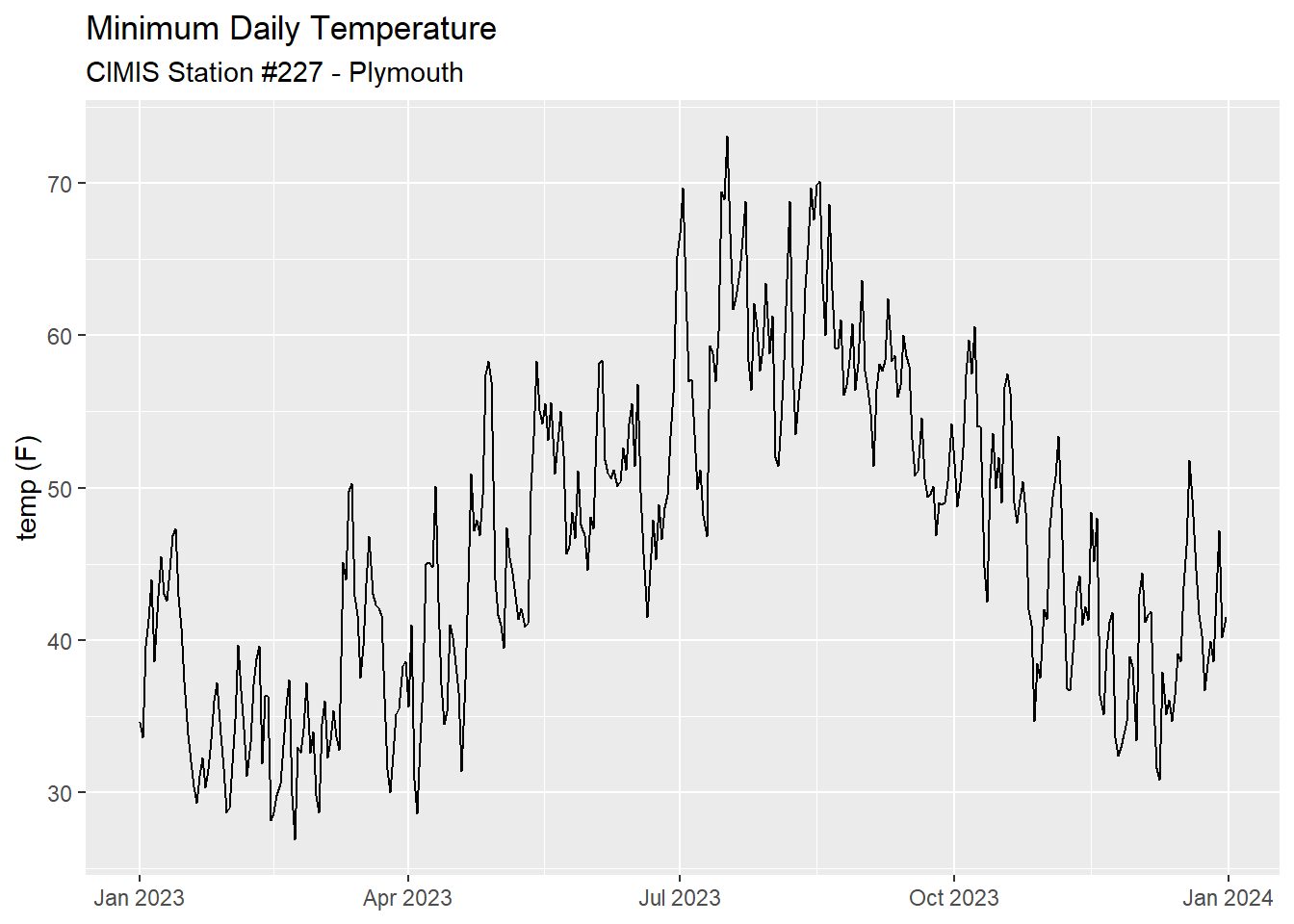
Visualize daily temperature

library(ggplot2)
ggplot(cimis227_dly_tbl, aes(x = date, y = tmin_f)) + 
  geom_line() + 
  xlab(NULL) +
  ylab("temp (F)") +
  labs(title = "Minimum Daily Temperature",
       subtitle = "CIMIS Station #227 - Plymouth")

2.2.2.3 CIMIS Hourly Data

CIMIS stations record measurements hourly. You can import hourly data with cimir, but the maximum number of records you can get from the API in one call is 1750 (about 5 months of data if you’re getting two variables every hour). Thus if you wanted an entire year of hourly data, you would have to make multiple calls for shorter periods and stack them together.

An alternative way to download hourly data is to use the CIMIS Station Reports tool on the CIMIS website. This tool allows you to specify station(s), start and end date(s), and weather variables. You can then get the data as a web report, csv, xml, or pdf.

Sign-in before generating CIMIS Station reports

To get the most options with CIMIS Station Reports, be sure to be logged-in with your CIMIS account. If you’re not logged in, you can still create station reports, but you’ll be limited to a few preset “limited reports”, which only go back 7 days and are only available to view in your browser.

Below, we’ll import a CIMIS Station Report containing one year of hourly air temperature and precipitation measurements for CIMIS station 227 - Plymouth (Amador County).

station_report_fn <- "./data/cimis_plymouth_station-report-2023.csv"

## Import the CSV file using readr and dplyr
cim_plymouth_hourly_tbl <- readr::read_csv(station_report_fn,
                                           col_types = "ncccccdcdc") |> 
  rename(stn_id = `Stn Id`, station_name = `Stn Name`, region = `CIMIS Region`,
         date_chr = Date, hour_pst = `Hour (PST)`, yday = Jul,
         precip_in = `Precip (in)`, precip_qc = `qc...8`,
         temp_f = `Air Temp (F)`, temp_qc = `qc...10`) |> 
  mutate(stn_id = as.character(stn_id))  ## for consistency with other datasets
New names:
• `qc` -> `qc...8`
• `qc` -> `qc...10`
head(cim_plymouth_hourly_tbl)


Next, we’ll create a cleaned-up version that we can save. First thing is to combine the Date and Hour columns into a R date-time class (POSIXct):

cimis227_hrly_tbl <- cim_plymouth_hourly_tbl |> 
  mutate(datetime = mdy_h(paste(date_chr, as.numeric(hour_pst) / 100), 
                          tz = "America/Los_Angeles")) 
Warning: There was 1 warning in `mutate()`.
ℹ In argument: `datetime = mdy_h(paste(date_chr, as.numeric(hour_pst)/100), tz
  = "America/Los_Angeles")`.
Caused by warning:
!  1 failed to parse.
head(cimis227_hrly_tbl)
Daylight Savings Time

When you’re switching the time zone of hourly data, you might get a parsing error if the time period includes the night when daylight savings time starts or ends.

The problem occurs because local time takes into account daylight savings. This is normally a good thing. However when the clock ‘falls back’, an entire hour of UTC time gets mapped onto the same local time. Similiarly on the night when you jump forward, 2:00am doesn’t exist in local time.

The workaround is to keep your data in UTC, or just ignore the warning.


Lastly, we can save the data as a csv file:

To save date-time values in CSV files (which are just text), a good practice is to format it in ISO8601 format, which is a well-established open standard for formatting time values as text, including timezone.

lubridate provides a function format_ISO8601() which makes this easy. The usetz argument appends the time offset from UTC, which import functions can use to figure out the time zone.

lubridate::format_ISO8601(Sys.time(), usetz = TRUE)
[1] "2024-02-10T16:29:13-0800"

You can import date-times formatted as ISO8601 back into R using lubridate::ymd_hms().

cimis227_hrly_tbl |> 
  mutate(dt = format_ISO8601(datetime, usetz = TRUE)) |> 
  select(stn_id, dt, temp_f, precip_in) |> 
  write_csv("./data/cimis227_hrly.csv")

To import these data into R, you can run one of the following:

Import from online (works from anywhere):

cimis227_hrly_tbl <- readr::read_csv("https://raw.githubusercontent.com/UCANR-IGIS/agroclimate-cookbook/main/data/cimis227_hrly.csv", col_types = "ccdd") |> 
  mutate(dt = lubridate::ymd_hms(dt, tz = "America/Los_Angeles"))

If you are working in the RStudio project for this e-book (e.g., authors):

cimis227_hrly_tbl <- readr::read_csv("./data/cimis227_hrly.csv", col_types = "ccdd") |> 
  mutate(dt = lubridate::ymd_hms(dt, tz = "America/Los_Angeles"))


2.2.3 Synoptic

Synoptic is an aggregator of weather data. The company grew out of a university project, and is now a public benefit corporation that offers access to weather data from over 140,000 weather stations across the USA. A notable feature of Synoptic is that they are not just a search engine. They actually host copies of the data and make them available to their customers thru their website and an API.

Synoptic hosts data from over 320 weather station networks, including several networks designed to support agriculture. To get an API key, sign-up for an account. The free account allows you to download historical data up to one year old.

Below, we’ll use a free account to get 4 months of data (March-June, 2023) for the Campo weather station in San Diego County. This station is managed by Western Weather Group on behalf of San Diego Gas and Electric.

There is no R package that provides functions to query the Synoptic API. But the API is well documented so we can use the httr2 package to make a call and parse the results.

First, let’s look at the metadata for this station:

library(httr2)

## Load token
my_public_token <- readLines("~/My Keys/synoptic-api.txt", n=1)

## You have to know the station id.
## Campo station ID: CPOSD

campo_meta_url <- paste0(
  "https://api.synopticdata.com/v2/stations/metadata?",
  "&token=", my_public_token,
  "&complete=1", 
  "&sensorvars=1",
  "&stid=CPOSD")

campo_meta_lst <- campo_meta_url |> 
  request() |> 
  req_perform() |> 
  resp_body_json()

lobstr::tree(campo_meta_lst)
<list>
├─STATION: <list>
│ └─<list>
│   ├─ID: "28759"
│   ├─STID: "CPOSD"
│   ├─NAME: "Campo"
│   ├─ELEVATION: "2433.0"
│   ├─LATITUDE: "32.59898"
│   ├─LONGITUDE: "-116.49292"
│   ├─STATUS: "ACTIVE"
│   ├─MNET_ID: "139"
│   ├─STATE: "CA"
│   ├─TIMEZONE: "America/Los_Angeles"
│   ├─ELEV_DEM: "2437.7"
│   ├─NWSZONE: "CA058"
│   ├─NWSFIREZONE: "SGX258"
│   ├─GACC: "SOCC"
│   ├─SHORTNAME: "SDGE"
│   ├─SGID: "SC11"
│   ├─COUNTY: "San Diego"
│   ├─COUNTRY: "US"
│   ├─WIMS_ID: <NULL>
│   ├─CWA: "SGX"
│   ├─PERIOD_OF_RECORD: <list>
│   │ ├─start: "2010-01-02T00:00:00Z"
│   │ └─end: "2024-02-12T05:30:00Z"
│   ├─PROVIDERS: <list>
│   │ ├─<list>
│   │ │ ├─name: "San Diego Gas and Electric"
│   │ │ └─url: "http://www.sdge.com/index/"
│   │ └─<list>
│   │   ├─name: "Western Weather Group"
│   │   └─url: "http://www.westernweathergroup.com"
│   ├─SENSOR_VARIABLES: <list>
│   │ ├─altimeter: <list>
│   │ │ └─altimeter_1: <list>
│   │ │   ├─position: "2.0"
│   │ │   └─PERIOD_OF_RECORD: <list>
│   │ │     ├─start: "2010-01-02T00:00:00Z"
│   │ │     └─end: "2013-03-14T19:10:00Z"
│   │ ├─pressure: <list>
│   │ │ └─pressure_1: <list>
│   │ │   ├─position: "2.0"
│   │ │   └─PERIOD_OF_RECORD: <list>
│   │ │     ├─start: "2010-01-02T00:00:00Z"
│   │ │     └─end: "2013-03-01T22:20:00Z"
│   │ ├─air_temp: <list>
│   │ │ └─air_temp_1: <list>
│   │ │   ├─position: "2.0"
│   │ │   └─PERIOD_OF_RECORD: <list>
│   │ │     ├─start: "2010-01-02T00:00:00Z"
│   │ │     └─end: "2024-02-12T05:30:00Z"
│   │ ├─relative_humidity: <list>
│   │ │ └─relative_humidity_1: <list>
│   │ │   ├─position: "2.0"
│   │ │   └─PERIOD_OF_RECORD: <list>
│   │ │     ├─start: "2010-01-02T00:00:00Z"
│   │ │     └─end: "2024-02-12T05:30:00Z"
│   │ ├─wind_speed: <list>
│   │ │ └─wind_speed_1: <list>
│   │ │   ├─position: "6.1"
│   │ │   └─PERIOD_OF_RECORD: <list>
│   │ │     ├─start: "2010-01-02T00:00:00Z"
│   │ │     └─end: "2024-02-12T05:30:00Z"
│   │ ├─wind_direction: <list>
│   │ │ └─wind_direction_1: <list>
│   │ │   ├─position: "6.1"
│   │ │   └─PERIOD_OF_RECORD: <list>
│   │ │     ├─start: "2010-01-02T00:00:00Z"
│   │ │     └─end: "2024-02-12T05:30:00Z"
│   │ ├─wind_gust: <list>
│   │ │ └─wind_gust_1: <list>
│   │ │   ├─position: "6.1"
│   │ │   └─PERIOD_OF_RECORD: <list>
│   │ │     ├─start: "2010-01-02T00:00:00Z"
│   │ │     └─end: "2024-02-12T05:30:00Z"
│   │ ├─solar_radiation: <list>
│   │ │ └─solar_radiation_1: <list>
│   │ │   ├─position: "6.1"
│   │ │   └─PERIOD_OF_RECORD: <list>
│   │ │     ├─start: "2010-01-02T00:00:00Z"
│   │ │     └─end: "2013-03-14T19:10:00Z"
│   │ └─volt: <list>
│   │   └─volt_1: <list>
│   │     ├─position: <NULL>
│   │     └─PERIOD_OF_RECORD: <list>
│   │       ├─start: "2019-09-12T19:43:00Z"
│   │       └─end: "2024-02-12T05:30:00Z"
│   ├─UNITS: <list>
│   │ ├─position: "m"
│   │ └─elevation: "ft"
│   └─RESTRICTED: FALSE
└─SUMMARY: <list>
  ├─NUMBER_OF_OBJECTS: 1
  ├─RESPONSE_CODE: 1
  ├─RESPONSE_MESSAGE: "OK"
  ├─METADATA_RESPONSE_TIME: "3.9 ms"
  └─VERSION: "v2.23.1"


To get weather data for a station, use the timeseries endpoint. Below we’ll get 4 months of data (March-June, 2023):

start_dt_utc_chr <- "202303010800"    ## must be in UTC (8 hours ahead)
end_dt_utc_chr <- "202307010700"      ## must be in UTC (7 hours ahead because of daylight savings)

campo_ts_url <- paste0("https://api.synopticdata.com/v2/stations/timeseries?token=", my_public_token,
                    "&stid=CPOSD",            ## CIMIS Station #152
                    "&vars=air_temp,relative_humidity,wind_speed",
                    "&varsoperator=and",      ## get all variables
                    "&units=english",         ## imperial units
                    "&start=", start_dt_utc_chr,  ## UTC time (+8)
                    "&end=", end_dt_utc_chr,      ## UTC time (+8)
                    "&obtimezone=local")      ## send back timestamps in local time

## Create a request object, make the call, and convert the results to a list
campo_ts_lst <- campo_ts_url |> 
  request() |> 
  req_perform() |> 
  resp_body_json()

The results include the timezone:

campo_ts_tz <- campo_ts_lst$STATION[[1]]$TIMEZONE
campo_ts_tz
[1] "America/Los_Angeles"

To convert the list into a data frame, we first pull out the individual observations:

## Get the date times for the time series
campo_ts_dt <- campo_ts_lst$STATION[[1]]$OBSERVATIONS$date_time |> 
  unlist() |> 
  ymd_hms(tz = campo_ts_tz)

campo_ts_airtemp_lst <- campo_ts_lst$STATION[[1]]$OBSERVATIONS$air_temp_set_1
campo_ts_airtemp_lst[sapply(campo_ts_airtemp_lst, length) == 0] <- NA
campo_ts_airtemp_vec <- campo_ts_airtemp_lst |> unlist()

campo_ts_rh_lst <- campo_ts_lst$STATION[[1]]$OBSERVATIONS$relative_humidity_set_1
campo_ts_rh_lst[sapply(campo_ts_rh_lst, length) == 0] <- NA
campo_ts_rh_vec <- campo_ts_rh_lst |> unlist()

campo_ts_ws_lst <- campo_ts_lst$STATION[[1]]$OBSERVATIONS$wind_speed_set_1
campo_ts_ws_lst[sapply(campo_ts_ws_lst, length) == 0] <- NA
campo_ts_ws_vec <- campo_ts_ws_lst |> unlist()

Now we have everything we need to build the tibble:

## Compute a tibble with the hourly values
campo2023_tbl <- tibble(dt = campo_ts_dt,
                         date = date(campo_ts_dt),
                         airtemp = campo_ts_airtemp_vec,
                         wind_speed = campo_ts_ws_vec,
                         rh = campo_ts_rh_vec)

head(campo2023_tbl)


Save as CSV:

write_csv(campo2023_tbl, file = "./data/campo2023.csv")

To use these data in examples, you can import the CSV file with either of the following:

Import from online (works from anywhere):

campo2023_tbl <- readr::read_csv("https://raw.githubusercontent.com/UCANR-IGIS/agroclimate-cookbook/main/data/campo2023.csv", 
                                 col_types = "cDddd") |> 
  mutate(dt = ymd_hms(dt, tz = "America/Los_Angeles"))


If you are working in the RStudio project for this e-book (e.g., authors), use:

campo2023_tbl <- readr::read_csv("./data/campo2023.csv", 
                                 col_types = "cDddd") |> 
  mutate(dt = ymd_hms(dt, tz = "America/Los_Angeles"))


2.2.4 gridMet & Prism

PRISM and gridMet are rasters of weather variables, interpolated from observed weather data.

gridMet is available via the Cal-Adapt API (up thru 2021?)

PRISM is available as NetCDF (I think). Only the 4k product is free.

Put these in Chapter 6 (will use stars to work with)


2.3 Cleaning Weather Data

2.3.1 Dealing with bad measurements

range checks

2.3.2 Missing data

see https://inresgb-lehre.iaas.uni-bonn.de/chillR_book/filling-gaps-in-temperature-records.html


2.4 Changing the Temporal Resolution of Weather Data

2.4.1 Short to Long

If you have timeseries data at short intervals (e.g. hourly), summarizing them by longer intervals (e.g., daily) is technically pretty straightforward using group_by() and summarise() from dplyr. However you have to think carefuly about which summary function is appropriate for the variable you’re interested in. The usual suspects are average, min, max.

Getting the time zone right

If you’re summarizing hourly data (or shorter) to daily intervals, and you’re using the traditional definition of a ‘day’ as starting and ending at midnight, then you’ll want to make sure your data are in local time. Otherwise you’ll be computing 24-hour summaries that start and end at 2pm (if your station is in the western USA, for example).

TODO: Give an example of using dplyr to group hourly CIMIS data into daily. Compare with the daily CIMIS data.

2.4.2 Interpolating Shorter Intervals

Going from daily values to hourly values,is less straightforward and requires a model for the downscaling. Most (all) weather variables don’t vary linearly over the course of the day, nor do they vary consistently over the seasons.

For more info, see:

https://inresgb-lehre.iaas.uni-bonn.de/chillR_book/making-hourly-temperatures.html